Field examples

Figure 8 is a seismic trace from marine survey. Figure 9a, 9b and 9c are the time-frequency distributions of the trace using local attribute (Liu et al., 2011), ensemble empirical mode decomposition and the proposed method. We can see that the energies distributions for ensemble empirical mode decomposition and the proposed method are much like each other. Both the ensemble empirical mode decomposition and the proposed method using the Hilbert transform of the intrinsic mode functions to represent the time-frequency distributions for the input signal. The results confirm that they both reveal the time-frequency character of the input signal.

trace
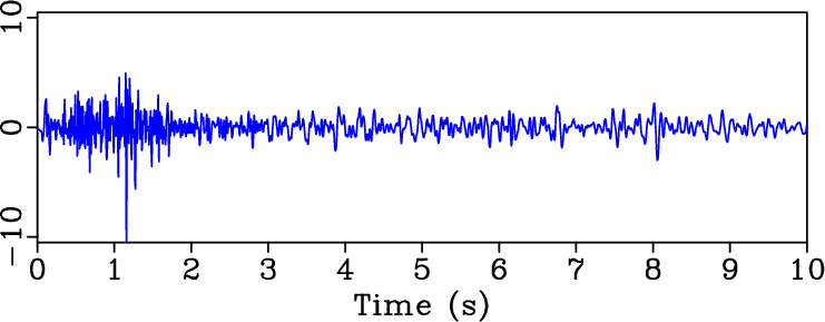
Figure 8. Seismic trace from marine survey.

stf,tfemd,tfnar
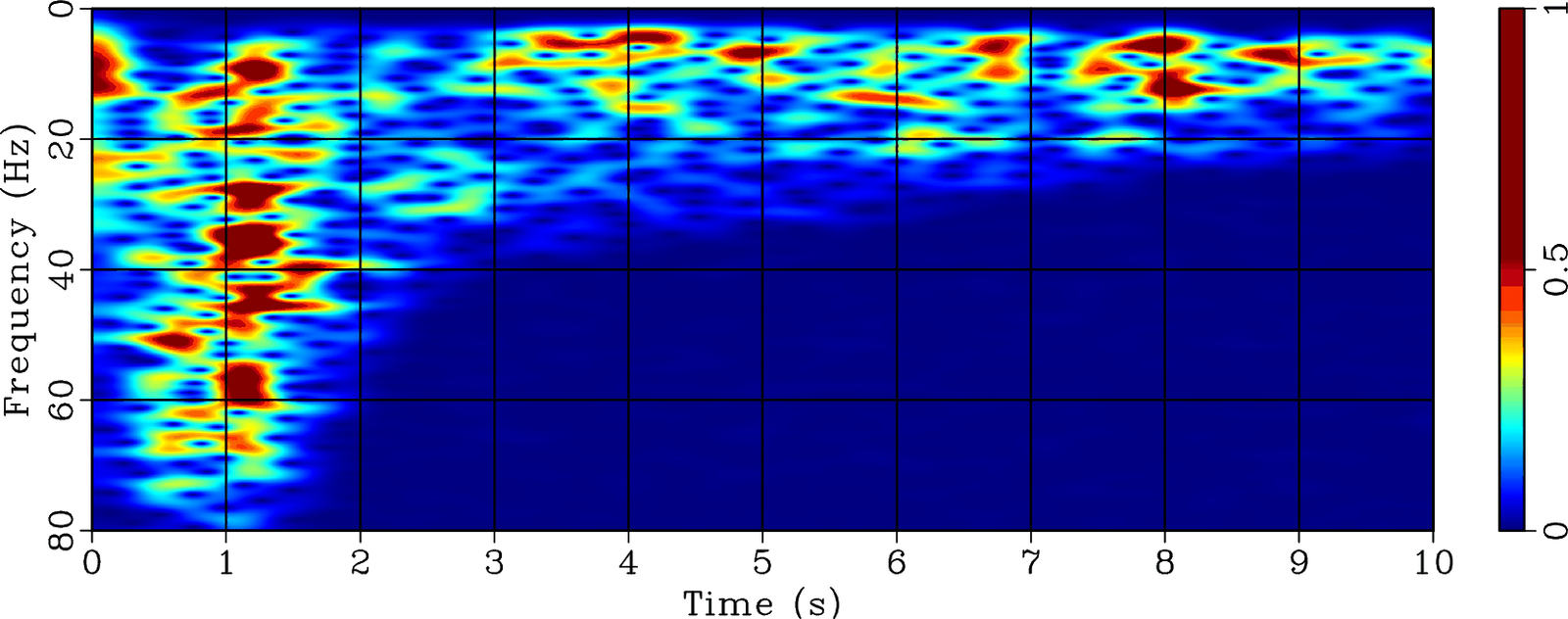
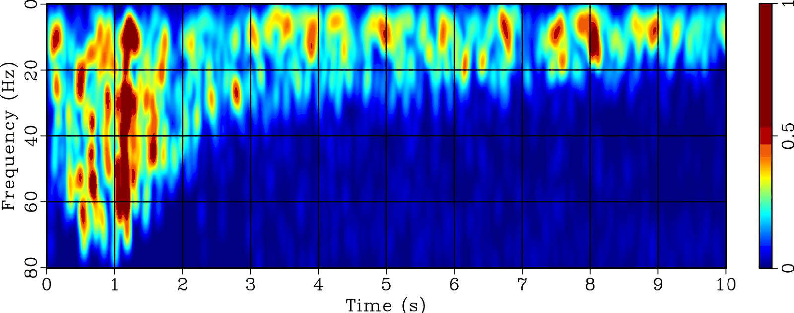
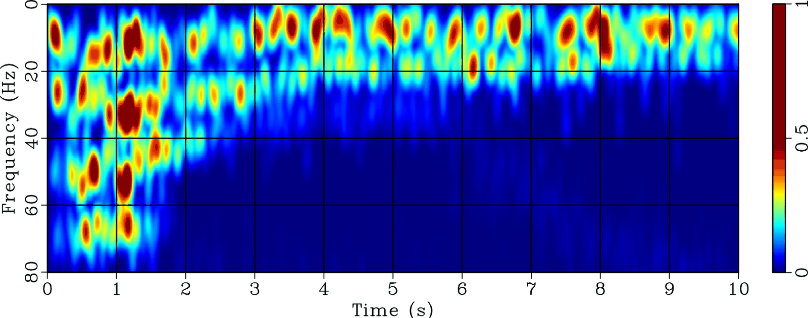
Figure 9. (a) Time-frequency map for synthetic signal of Figure 8 using local attribute. (b) Time-frequency map for synthetic signal of Figure 8 using ensemble empirical mode decomposition. (c) Time-frequency map for synthetic signal of Figure 8 using the proposed method.

Low-frequency anomalies are often attributed to abnormally high attenuation in gas-filled reservoirs and can be used as a hydrocarbon indicator (Castagna et al., 2003). The mechanisms of low-frequency anomalies associated with hydrocarbon reservoirs are not clearly understood (Kazemeini et al., 2009; Ebrom, 2004). Figure 10 is a 2D field seismic data. Figure 11a and 11b,  11c and 11d,  11e and 11f are the 30Hz and 60Hz constant frequency slices using local attribute, ensemble empirical mode decomposition and the proposed method. From the above figures, we see that there is a low frequency anomaly in the upper left part of the data section indicated by the text boxes "Gas?" for the ensemble empirical mode decomposition and the proposed methods, which may correspond to gas presentation.

data
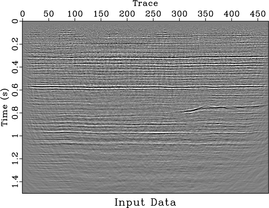
Figure 10. 2D seismic data section.

LC_TimeFreqSlice3,LC_TimeFreqSlice6,GasSmoothSliceEmd3,GasSmoothSliceEmd6,GasSmoothSliceNar3,GasSmoothSliceNar6
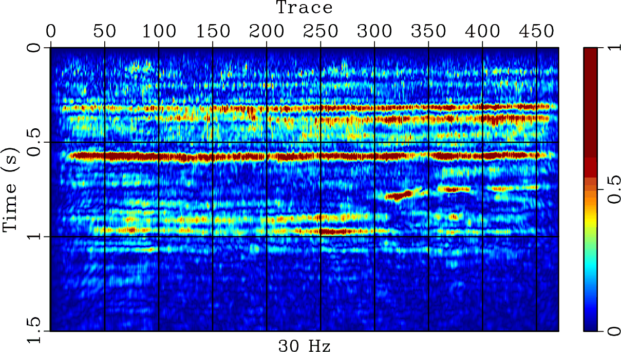
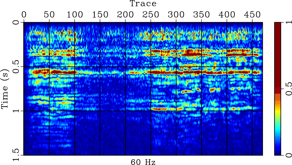
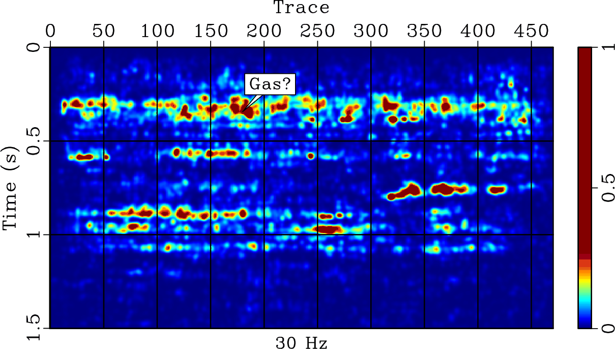
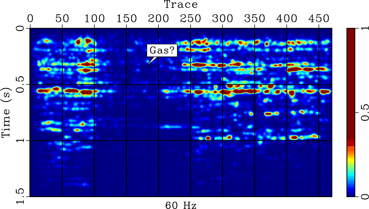
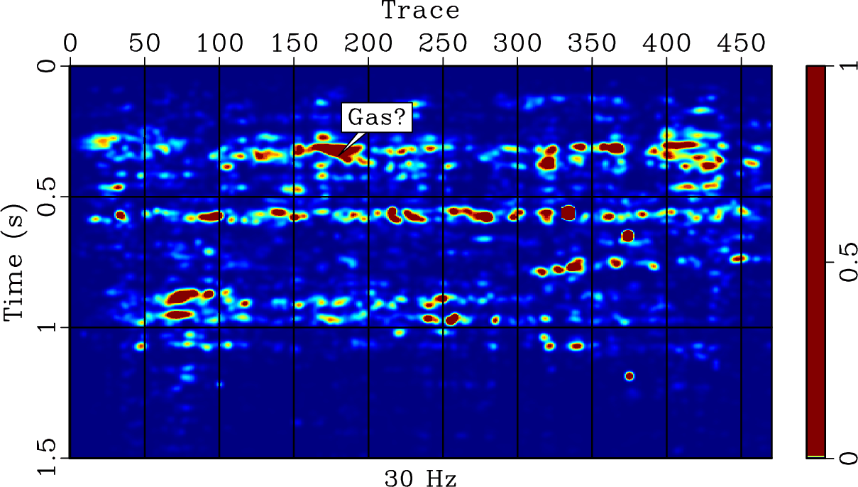
Figure 11. (a) 30Hz slice time-frequency map using local attribute method. (b) 60Hz slice time-frequency map using local attribute method. (c) 30Hz slice time-frequency map using ensemble empirical mode decomposition method. (d) 60Hz slice time-frequency map using ensemble empirical mode decomposition method. (e) 30Hz slice time-frequency map of the proposed method. (f) 60Hz slice time-frequency map of the proposed method.

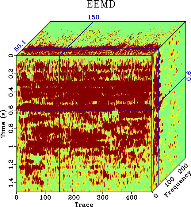
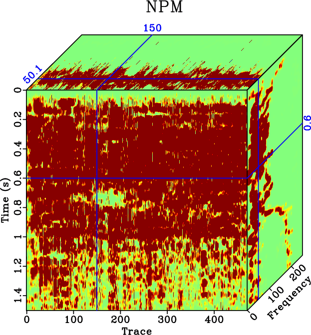
Figure 12a, 12b and 12c are the full time-frequency cubes computed respectively using local attribute, ensemble empirical mode decomposition and the proposed methods. The main panels show constant frequency slices. The right hand side panels show the time-frequency maps of the 150th trace. The top panels show the time-frequency maps of 0.6s time-depth signal. From the right and top side panels we see that there are a lot of noise in the high frequency domain for the ensemble empirical mode decomposition and local attribute methods compared with the proposed method.

TimeFreqCube_LC,TimeFreqCubeEmd,TimeFreqCubeNar
Figure 12. (a) Time-frequency cube using local attribute method. (b) Time-frequency cube using ensemble empirical mode decomposition method. (c) Time-frequency cube using NPM method.