|
|
|
|
Fast Streaming Local Time-frequency Transform for Nonstationary Seismic Data Processing |
Next: Fast Multicomponent Data Registration Up: Applications Previous: Fast Ground-roll Attenuation in
|
|
|
|
Fast Streaming Local Time-frequency Transform for Nonstationary Seismic Data Processing |
Local Time-frequency map can also used for time-varying Q-factor
estimation and inverse-Q filtering. Wang et al. (2020) developed the
local centroid frequency shift (LCFS) method for time-varying
Q-estimation in time-frequency domain. The SLTFT method can provide
accurate time-frequency spectrum for Q-factor estimation with high
efficiency. We selected a 2D poststack seismic profile to perform
numerical test (see Fig.10a). The seismic
section has a time length of 4.5 s with a time sampling of 4 ms and
contains 247 traces in total. We calculated the
 spectrum of the seismic section (see
Fig.10b) by using the SLTFT
(
spectrum of the seismic section (see
Fig.10b) by using the SLTFT
(
 ). The spectrum shows that the frequency range is
getting narrow as the seismic wave propagates. The local centroid
frequency (LCF) can be calculated by using the
map (Liu and Fomel, 2013; Wang et al., 2020), as is shown in
Fig.10c. We used the LCFS method in
time-frequency domain to estimate the time-varying equivalent
Q-factors for each
trace. Fig.11a-11c
show the calculated Q-factors by using the S transform, the LTF
decomposition and the SLTFT, respectively. The Q-factors obtained by
the LTF decomposition and the SLTFT are reasonably distributed
according to the LCF information (see Fig.10c),
while the S-transform fails in providing an unbiased Q-factor map. The
estimated Q-factors are used to perform inverse-Q filtering, and
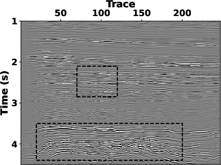
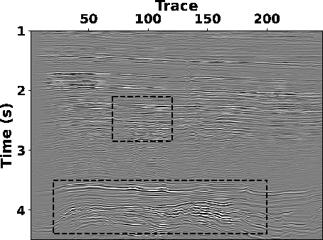
Fig.12a - 12c show
the enhanced seismic sections corresponded to
Fig.11a-11c,
respectively. Because of its biased estimation of Q-factors, the
S-transform exhibits limitations in effectively enhancing the
resolution of deep reflection signals (around 3
). The spectrum shows that the frequency range is
getting narrow as the seismic wave propagates. The local centroid
frequency (LCF) can be calculated by using the
map (Liu and Fomel, 2013; Wang et al., 2020), as is shown in
Fig.10c. We used the LCFS method in
time-frequency domain to estimate the time-varying equivalent
Q-factors for each
trace. Fig.11a-11c
show the calculated Q-factors by using the S transform, the LTF
decomposition and the SLTFT, respectively. The Q-factors obtained by
the LTF decomposition and the SLTFT are reasonably distributed
according to the LCF information (see Fig.10c),
while the S-transform fails in providing an unbiased Q-factor map. The
estimated Q-factors are used to perform inverse-Q filtering, and
Fig.12a - 12c show
the enhanced seismic sections corresponded to
Fig.11a-11c,
respectively. Because of its biased estimation of Q-factors, the
S-transform exhibits limitations in effectively enhancing the
resolution of deep reflection signals (around 3  4 s) (see
Fig.12a) when compared to the results of the
LTF decomposition and the SLTFT (see Fig.12b
and 12c), where the attenuation of the
reflections is compensated well, and the original structural
characteristics are reasonably preserved. Meanwhile, the proposed
method effectively reduces more computational costs (see
Table. 2) than the LTF decomposition. Additionally,
it achieves storage cost reduction through flexible frequency
down-sampling. Specifically, in the SLTFT, we utilize half the
frequency samples compared to the S-transform, while maintaining a
superior enhancing profile.
4 s) (see
Fig.12a) when compared to the results of the
LTF decomposition and the SLTFT (see Fig.12b
and 12c), where the attenuation of the
reflections is compensated well, and the original structural
characteristics are reasonably preserved. Meanwhile, the proposed
method effectively reduces more computational costs (see
Table. 2) than the LTF decomposition. Additionally,
it achieves storage cost reduction through flexible frequency
down-sampling. Specifically, in the SLTFT, we utilize half the
frequency samples compared to the S-transform, while maintaining a
superior enhancing profile.


|
|---|
|
powdata,sltft0,ltft_cf
Figure 10. (a) 2D poststack seismic section, (b) the corresponding cube
and (c) local centroid frequency.
|
|
|


|
|---|
|
st_eqvq,ltft_eqvq,sltft_eqvq
Figure 11. The estimated equivalent Q-factors by using (a) S-transform, (b) LTF decomposition and (c) SLTFT ( ).
|
|
|

|
|---|
|
stresult,ltftresult,sltftresult
Figure 12. Enhanced seismic sections by using (a) S-transform, (b) LTF decomposition and (c) SLTFT ( ).
|
|
|
|
|
|
|
Fast Streaming Local Time-frequency Transform for Nonstationary Seismic Data Processing |