Homework 3

Fourier compression

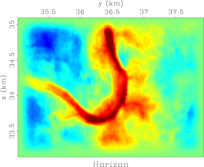
In this exercise, we will use a depth slice selected from a 3-D seismic volume and shown in Figure 3 (Hall, 2007). Notice a channel structure.

data Figure 3. Seismic depth slice with a channel structure.

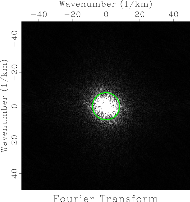
fft Figure 4. Absolute value of the Fourier transform of the seismic slice from Figure 3. The circle inside shows a window selected for compression.

The goal of your assignment is to find a compressed representation of the data in the Fourier transform domain. Figure 4 shows the Fourier transform of the data from Figure 3. We can see that most of the energy gets concentrated near the center (zero frequency).

There are two alternative ways to compress data in the Fourier domain:

• One approach is to select a range of frequencies that contain the most important information. An advantage of this approach is the ability to subsample the original data by transforming back from a windowed range of frequencies. The results from this method are shown in Figure 5.
• Another approach is to zero all Fourier coefficients below a certain threshold value, regardless of which frequencies they represent. The results from this method are shown in Figure 6. Figure 7 shows the selected threshold plotted against the histogram of Fourier coefficients.

sig,cut
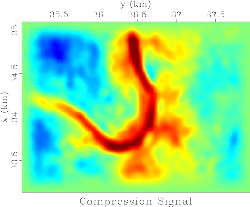
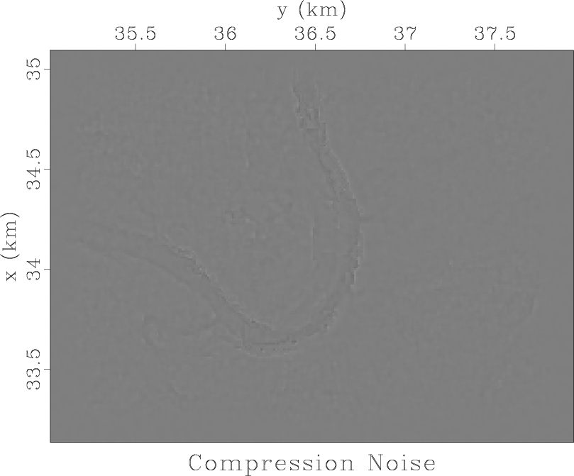
Figure 5. Data separated into signal (a) and noise (b) by applying Fourier compression with windowing.

thr,noi
Figure 6. Data separated into signal (a) and noise (b) by applying Fourier compression with thresholding.

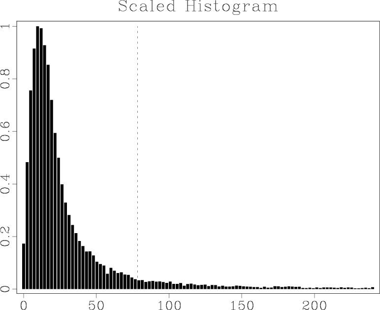
hist Figure 7. Normalized histogram of Fourier coefficients (by absolute value). The vertical line shows the selected threshold.

1. Change directory to hw3/compress.
2. Run

   scons view
   

   to reproduce the figures on your screen.
3. Modify the SConstruct file to decrease the size of the window so that the noise level increases in Figure 5b. How do you measure the noise level? Find a level that you find negligibly small.
4. Modify the SConstruct file to increase the threshold value so that the compression achieves the same quality as in the previous case. The noise level in Figure 6b should match that in Figure 5b.
5. Compare the number of nonzero Fourier coefficients in both cases. Which method achieves a better compression?
6. EXTRA CREDIT for finding a way for a better compression of the data in the Fourier domain. Your data reconstruction should have the same noise level, yet the number of non-zero coefficients in the Fourier domain should be smaller.

from rsf.proj import *

# Get data
##########
Fetch('horizon.asc','hall')

# Convert format
Flow('data','horizon.asc',
     '''
     echo in=$SOURCE data_format=ascii_float n1=3 n2=57036 | 
     dd form=native | window n1=1 f1=-1 | add add=-65 | 
     put 
     n2=291 o2=35.031 d2=0.01 label2=y unit2=km 
     n1=196 o1=33.139 d1=0.01 label1=x unit1=km |
     costaper nw1=25 nw2=25 
     ''')

# Display
def plot(title):
    return '''
    grey color=j title="%s" 
    transp=y yreverse=n clip=14
    ''' % title
Result('data',plot('Horizon'))

# 2-D Fourier Transform
#######################
Flow('fft','data',
     'rtoc | fft3 axis=1 pad=1 | fft3 axis=2 pad=1')
Plot('fft',
     '''
     math output="abs(input)" | real | 
     grey title="Fourier Transform" allpos=y screenratio=1
     ''')

# A. Compression by Windowing
#############################

cut = 8 # !!! CHANGE ME !!!

# Create a frame
Flow('frame','fft','real | math output="sqrt(x1*x1+x2*x2)" ')
Plot('frame',
     '''
     contour nc=1 c0=%g plotfat=5 plotcol=3
     wantaxis=n wanttitle=n screenratio=1
     ''' % cut)
Result('fft','fft frame','Overlay')

# Cut a hole
Flow('fcut','frame fft',
     '''
     mask max=%g | 
     dd type=float | rtoc |
     mul ${SOURCES[1]}
     ''' % cut)

# Inverse FFT
Flow('sig','fcut',
     'fft3 axis=2 inv=y | fft3 axis=1 inv=y | real')
Result('sig',plot('Compression Signal'))

Flow('cut','data sig','add scale=1,-1 ${SOURCES[1]}')
Result('cut',plot('Compression Noise') + 'color=I')

# B. Compression by Thresholding
################################

thr = 80 # !!! CHANGE ME !!!

# Plot histogram
Plot('hist','fft',
     '''
     math output="abs(input)" | real |
     histogram o1=0 d1=%g n1=101 |
     dd type=float | scale axis=1 |
     bargraph title="Scaled Histogram" pad1=n
     label1= unit1= label2= unit2=
     ''' % (0.03*thr))
Flow('line.asc',None,
     'echo 0 0 0 1 n1=4 data_format=ascii_float in=$TARGET')
Plot('line','line.asc',
     '''
     dd type=complex form=native | 
     graph min1=-1 max1=2 plotcol=5 
     wantaxis=n wanttitle=n dash=1
     ''')
Result('hist','hist line','Overlay')

# Thresholding
Flow('fthr','fft','thr thr=%g' % thr)

# Inverse FFT
Flow('thr','fthr',
     'fft3 axis=2 inv=y | fft3 axis=1 inv=y | real')
Result('thr',plot('Compression Signal'))

# Subtract from Data
Flow('noi','data thr','add scale=1,-1 ${SOURCES[1]}')
Result('noi',plot('Compression Noise') + 'color=I')

End()

Homework 3