Interpolation after coordinate transformation

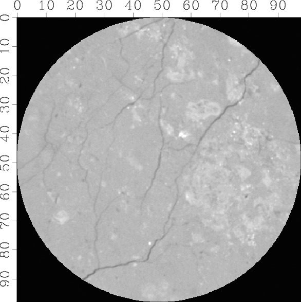
In this exercise, we will use a slice out of a 3-D CT-scan of a carbonate rock sample, shown in Figure 1a . Notice microfracture channels.


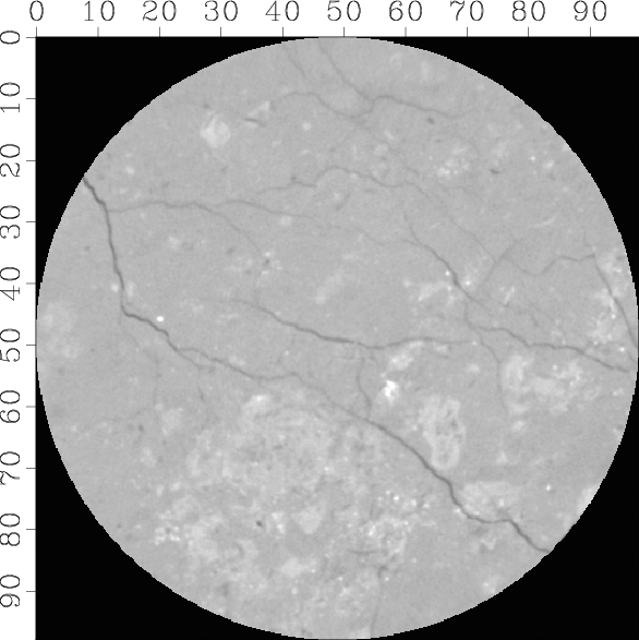
circle,rotate Figure 1. Slice of a CT-scan of a carbonate rock sample. (a) Original. (b) After clockwise rotation by $90^{\circ }$ .

The goal of the exercise is to apply a coordinate transformation to the original data. A particular transformation that we will study is coordinate rotation. Figure 1b shows the original slice rotated by 90 degrees. A 90-degree rotation in this case amounts to simple transpose. However, rotation by a different angle requires interpolation from the original grid to the modified grid.

The task of coordinate rotation is accomplished by the C program rotate.c (alternatively, Python script rotate.py.) Two different methods are implemented: nearest-neighbor interpolation and bilinear interpolation.

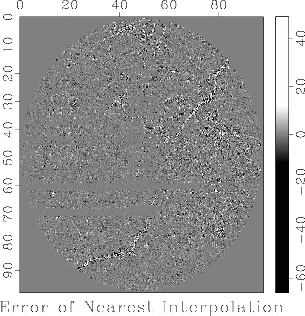
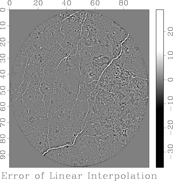
To test the accuracy of different methods, we can rotate the original data in small increments and then compare the result of rotating to $360^{\circ}$ with the original data. Figure 2 compares the error of the nearest-neighbor and bilinear interpolations after rotating the original slice in increments of $20^{\circ}$ . The accuracy is comparatively low for small discontinuous features like microfracture channels.

To improve the accuracy further, we need to employ a longer filter. One popular choice is cubic convolution interpolation, invented by Robert Keys (a geophysicist, currently at ConocoPhillips). The cubic convolution filter can be expressed as the filter (Keys, 1981)


nearest,linear Figure 2. Error of different interpolation methods computed after full circle rotation in increments of 20 degrees. (a) Nearest-neighbor interpolation. (b) Bi-linear interpolation.

/* Rotate around. */
#include <rsf.h>

int main(int argc, char* argv[])
{
    int n1, n2, i1, i2, k1, k2;
    float x1, x2, c1, c2, cosa, sina, angle;
    float **orig, **rotd;
    char *interp;
    sf_file inp, out;

    /* initialize */
    sf_init(argc,argv);
    inp = sf_input("in");
    out = sf_output("out");

    /* get dimensions from input */
    if (!sf_histint(inp,"n1",&n1)) sf_error("No n1= in inp");
    if (!sf_histint(inp,"n2",&n2)) sf_error("No n2= in inp");

    /* get parameters from command line */
    if (!sf_getfloat("angle",&angle)) angle=90.;
    /* rotation angle */

    if (NULL == (interp = sf_getstring("interp"))) 
	interp="nearest";
    /* [n,l,c] interpolation type */

    /* convert degrees to radians */
    angle *= SF_PI/180.;
    cosa = cosf(angle);
    sina = sinf(angle);

    orig = sf_floatalloc2(n1,n2);
    rotd = sf_floatalloc2(n1,n2);

    /* read data */
    sf_floatread(orig[0],n1*n2,inp);

    /* central point */
    c1 = (n1-1)*0.5;
    c2 = (n2-1)*0.5;

    for (i2=0; i2 < n2; i2++) {
	for (i1=0; i1 < n1; i1++) {

	    /* rotated coordinates */
	    x1 = c1+(i1-c1)*cosa-(i2-c2)*sina;
	    x2 = c2+(i1-c1)*sina+(i2-c2)*cosa;

	    /* nearest neighbor */
	    k1 = floorf(x1); x1 -= k1;
	    k2 = floorf(x2); x2 -= k2;

	    switch(interp[0]) {
		case 'n': /* nearest neighbor */
		    if (x1 > 0.5) k1++;
		    if (x2 > 0.5) k2++;
		    if (k1 >=0 && k1 < n1 &&
			k2 >=0 && k2 < n2) {
			rotd[i2][i1] = orig[k2][k1];
		    } else {
			rotd[i2][i1] = 0.;
		    }
		    break;
		case 'l': /* bilinear */
		    if (k1 >=0 && k1 < n1-1 &&
			k2 >=0 && k2 < n2-1) {
			rotd[i2][i1] = 
			    (1.-x1)*(1.-x2)*orig[k2][k1]   +
			    x1     *(1.-x2)*orig[k2][k1+1] +
			    (1.-x1)*x2     *orig[k2+1][k1] +
			    x1     *x2     *orig[k2+1][k1+1];
		    } else {
			rotd[i2][i1] = 0.;
		    }
		    break;
		case 'c': /* cubic convolution */
		    /* !!! ADD CODE !!! */
		    break;
		default:
		    sf_error("Unknown method %s",interp);
		    break;
	    }
	}
    }

    /* write result */
    sf_floatwrite(rotd[0],n1*n2,out);

    exit(0);
}

#!/usr/bin/env python

import sys
import math
import numpy as np
import m8r

# initialize
par = m8r.Par()
inp = m8r.Input()
out = m8r.Output()

# get dimensions from input
n1 = inp.int('n1')
n2 = inp.int('n2')

# get parameters from command line
angle = par.float('angle',90.)
# rotation angle

interp = par.string('interp','nearest')
# [n,l,c] interpolation type 

# convert degrees to radians
angle = angle*math.pi/180.
cosa = math.cos(angle)
sina = math.sin(angle)

orig = np.zeros([n1,n2],'f')
rotd = np.zeros([n1,n2],'f')

# read data
inp.read(orig)

# central point 
c1 = (n1-1)*0.5
c2 = (n2-1)*0.5

for i2 in range(n2):
    for i1 in range(n1):
        # rotated coordinates
        x1 = c1+(i1-c1)*cosa-(i2-c2)*sina
        x2 = c2+(i1-c1)*sina+(i2-c2)*cosa

	    # nearest neighbor
        k1 = int(math.floor(x1))
        k2 = int(math.floor(x2))
        x1 -= k1	    
        x2 -= k2

        if interp[0] == 'n':
            # nearest neighbor
            if x1 > 0.5:
                k1 += 1
            if x2 > 0.5:
                k2 += 1
            if k1 >=0 and k1 < n1                and k2 >=0 and k2 < n2:
                rotd[i2,i1] = orig[k2,k1]
            else:
                rotd[i2,i1] = 0.
        elif interp[0] == 'l':
            # bilinear
            if k1 >=0 and k1 < n1-1                and k2 >=0 and k2 < n2-1:
                rotd[i2,i1] =  			    (1.-x1)*(1.-x2)*orig[k2,k1]   +  			    x1     *(1.-x2)*orig[k2,k1+1] +  			    (1.-x1)*x2     *orig[k2+1,k1] +  			    x1     *x2     *orig[k2+1,k1+1]
            else:
                rotd[i2,i1] = 0.
        elif interp[0] == 'c':
            # cubic convolution 
		    # !!! ADD CODE !!!
            break
        else:
            sys.stderr.write('Unknown method "%s"' % interp)
            sys.exit(1)

 # write result */
out.write(rotd)
sys.exit(0)

from rsf.proj import *

# Download data
Fetch('slice.rsf','ctscan')
Flow('circle','slice','dd type=float')

grey = 'grey wanttitle=n screenratio=1 bias=128 clip=105'

Result('circle',grey)

# Rotate program
# exe = Program('rotate.c')

# UNCOMMENT ABOVE AND COMMENT BELOW IF YOU WANT TO USE C 
exe = Command('rotate.exe','rotate.py','cp $SOURCE $TARGET')
AddPostAction(exe,Chmod(exe,0o755))

rotate = str(exe[0])

# Rotate by 90 degrees
Flow('rotate',['circle',rotate],
     './${SOURCES[1]} angle=90 interp=nearest')

Result('rotate',grey)

# Mask for the circle
Flow('mask','circle',
     '''
     put d1=1 o1=-255.5 d2=1 o2=-255.5 |
     math output="sqrt(x1*x1+x2*x2)" |
     mask min=255.5 | dd type=float | 
     smooth rect1=3 rect2=3 |
     mask max=0 | dd type=float |
     put d1=0.1914 o1=0 d2=0.1914 o2=0
     ''')

for case in ('nearest','linear'): # !!! MODIFY ME !!!
    new = 'circle'
    rotates = []
    for r in range(18):
        old = new
        new = '%s-circle%d' % (case,r)
        Flow(new,[old,rotate],
             './${SOURCES[1]} angle=20 interp=%s' % case)
        Plot(new,grey)
        rotates.append(new)

    # Movie of rotating circle
    Plot(case,rotates,'Movie',view=1)

    # Plot error
    Result(case,[new,'circle','mask'],
           '''
           add scale=1,-1 ${SOURCES[1]} |
           add mode=p ${SOURCES[2]} |
           %s bias=0 scalebar=y clip=12
           wanttitle=y title="Error of %s Interpolation"
           ''' % (grey,case.capitalize()))

End()

$\displaystyle Z^{\sigma} \approx C(Z)$	$\textstyle =$	$\displaystyle -\frac{\sigma (1-\sigma)^2}{2} Z^{-1} + \frac{(1-\sigma) (2 + 2 \sigma - 3 \sigma^2)}{2} +$
		$\displaystyle \frac{\sigma (1 + 4 \sigma - 3 \sigma^2)}{2} Z - \frac{(1-\sigma) \sigma^2}{2} Z^2\;.$	(8)