Homework 3

Projection onto convex sets

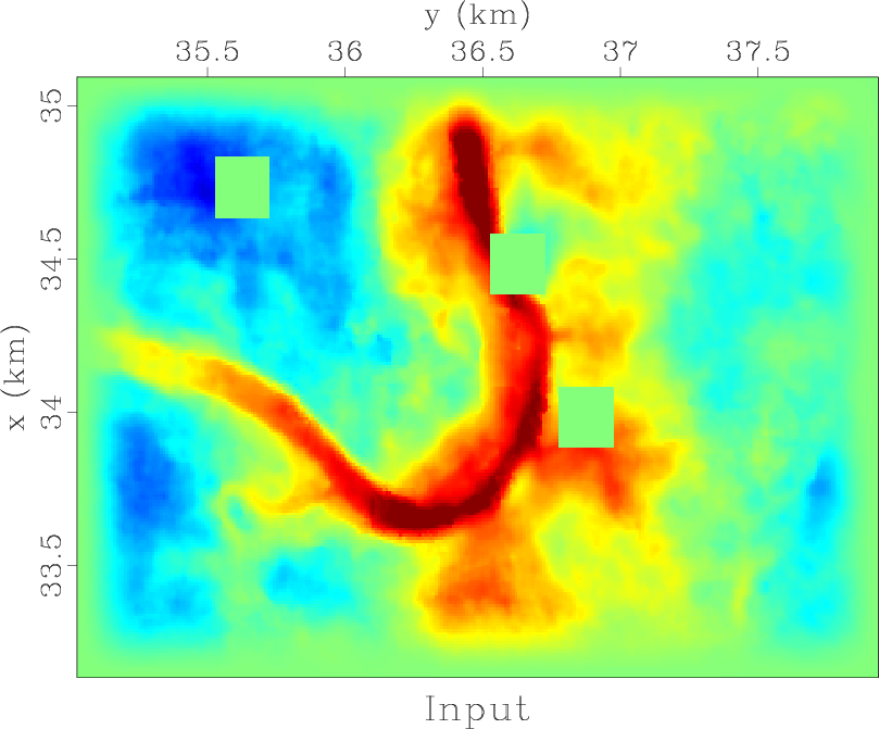
hole Figure 8. Seismic depth slice after removing selected parts of the data.

The goal of the next exercise is to figure out if one can use compactness of the Fourier transform to reconstruct missing data. The missing parts are created artificially by cutting holes in the original data (Figure 8).

fft-data,fft-hole
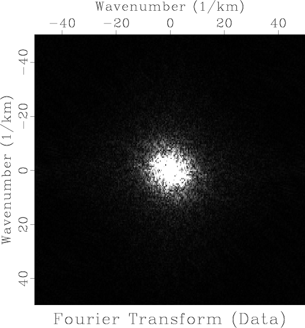
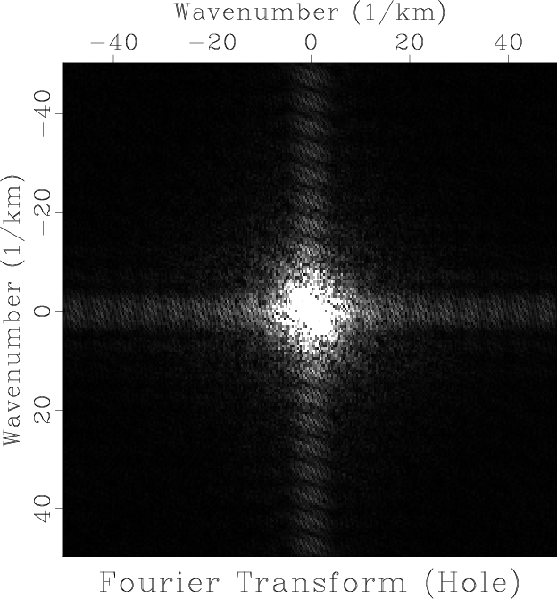
Figure 9. Fourier transform of the original data (a) and data with holes with holes (b). The absolute value is displayed

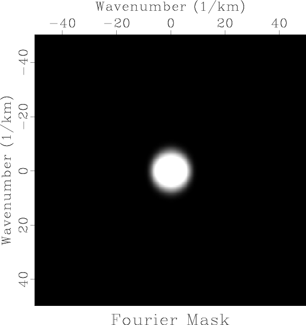
fft-mask Figure 10. Fourier-domain mask for selecting a convex set.

Figures 9a and 9b show the digital Fourier transform of the original data and the data with holes. We observe again that the support of the data in the Fourier domain is compact thanks to the data smoothness. Cutting holes in the physical domain creates discontinuities that make the Fourier response spread beyond the original support. Figure 10 shows a Fourier-domain mask designed to contain the support of the original data.

To accomplish the task of missing data interpolation, we will use an iterative method known as POCS (projection onto convex sets). By definition, a convex set $\mathcal{C}$ is a set of functions such that, for any $f_1(\mathbf{x})$ and $f_2(\mathbf{x})$ from the set, $g(\mathbf{x}) = \lambda f_1(\mathbf{x}) + (1-\lambda) f_2(\mathbf{x})$ (for $0 \le \lambda \le 1$) also belongs to the set. A projection onto a convex set means finding a function in the set that is of the shortest distance to the given function. The POCS theorem states that if one wants to find a function that belongs to the intersection of two convex sets $C_1$ and $C_2$, the task can be accomplished iteratively by alternating projections onto the two sets (Youla and Webb, 1982).

In our example, $C_1$ is the set of all functions that are equal to the known data outside of the holes. $C_2$ is the set of all functions that have a predifined compact support in the Fourier domain (and therefore are smooth in the physical domain). The algorithm consists of the following steps:

1. Apply 2-D Fourier transform.
2. Multiply by a Fourier-transform mask to enforce compact support.
3. Apply inverse 2-D Fourier transform.
4. Replace data outside of the holes with known data.
5. Repeat.

The output after 5 iterations is shown in Figure 11.

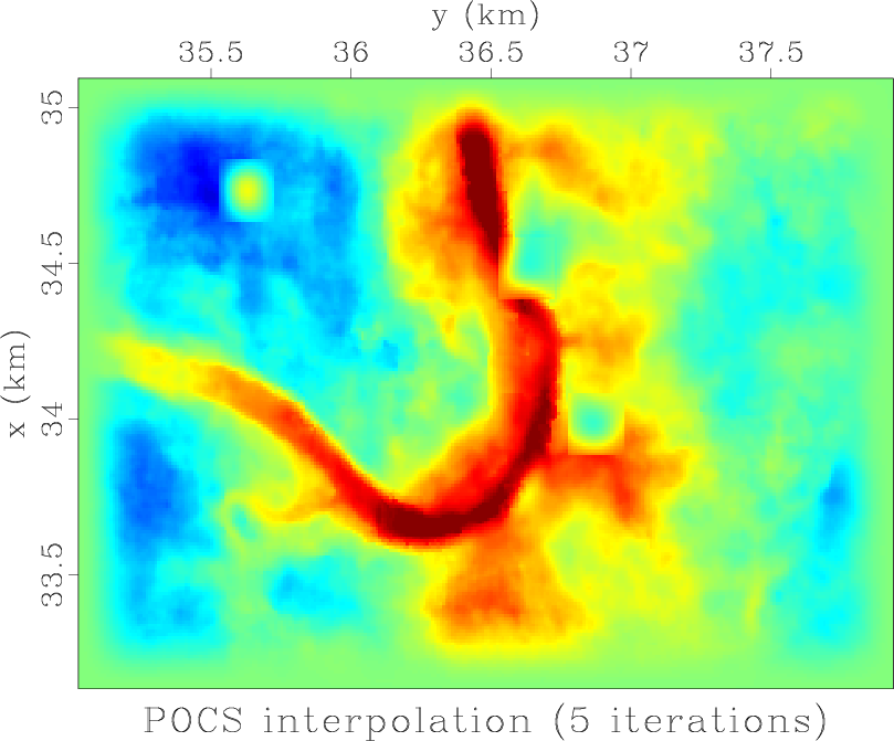
pocs Figure 11. Missing data interpolated by iterative projection onto convex sets.

from rsf.proj import *

# Download data
Fetch('horizon.asc','hall')

# Convert format
Flow('data','horizon.asc',
     '''
     echo in=$SOURCE data_format=ascii_float n1=3 n2=57036 | 
     dd form=native | window n1=1 f1=-1 | add add=-65 | 
     put 
     n2=291 o2=35.031 d2=0.01 label2=y unit2=km 
     n1=196 o1=33.139 d1=0.01 label1=x unit1=km |
     costaper nw1=25 nw2=25 
     ''')

# Display
def plot(title):
    return '''
    grey color=j title="%s" 
    transp=y yreverse=n clip=14
    ''' % title
Result('data',plot('Horizon'))

# Cut three square holes (!!! CHANGE ME !!!)
cut = '''
cut n1=20 n2=20 f1=125 f2=150 | 
cut n1=20 n2=20 f1=150 f2=50  | 
cut n1=20 n2=20 f1=75  f2=175
'''

Flow('hole','data',cut)
Flow('mask','data',
     'math output=1 | %s | math output=1-input' % cut)
Plot('hole',plot('Input'))
Result('hole','Overlay')

# Fourier transform
forw = 'rtoc | fft3 axis=1 pad=1 | fft3 axis=2 pad=1'
back = 'fft3 axis=2 inv=y | fft3 axis=1 inv=y | real'

for data in ('data','hole'):
    fft = 'fft-'+data
    Flow(fft,data,forw)
    Result(fft,
           '''
           math output="abs(input)" | real | 
           grey allpos=y title="Fourier Transform (%s)" 
           screenratio=1
           ''' % data.capitalize())

# Create Fourier mask
Flow('fft-mask','fft-hole',
     '''
     real | math output="x1*x1+x2*x2" | mask min=50 |
     dd type=float | math output=1-input | 
     smooth rect1=5 rect2=5 repeat=3 | rtoc
     ''')
Result('fft-mask',
       '''
       real | 
       grey allpos=y title="Fourier Mask" screenratio=1
       ''')

# POCS iterations
niter=5 # !!! CHANGE ME !!!

data = 'hole'
plots = ['hole']
for iter in range(niter): 
    old = data
    data = 'data%d' % iter

    # 1. Forward FFT
    # 2. Multiply by Fourier mask
    # 3. Inverse FFT
    # 4. Multiply by space mask
    # 5. Add data outside of hole
    Flow(data,[old,'fft-mask','mask','hole'],
         '''
         %s | mul ${SOURCES[1]} | 
         %s | mul ${SOURCES[2]} | 
         add ${SOURCES[3]}
         ''' % (forw,back))
    Plot(data,plot('Iteration %d' % (iter+1)))
    plots.append(data)
# Put frames in a movie
Plot('pocs',plots,'Movie',view=1)

# Last frame
Result('pocs',data,
       plot('POCS interpolation (%d iterations)' % niter))

End()

Your task:

1. Change directory to hw3/pocs
2. Run

   scons view
   

   to reproduce the figures on your screen.
3. Additionally, you can run

   scons pocs.vpl
   

   to see a movie of different iterations.
4. By modifying appropriate parameters in the SConstruct file and repeating computations, find out
   1. How many iterations are required for convergence?
   2. How large can you make the holes and still be able to achieve a reasonably good reconstruction?
5. EXTRA CREDIT for finding a different convex set for either faster or more accurate missing data reconstruction.

Homework 3