A new paper is added to the collection of reproducible documents:
Stratigraphic coordinates, a coordinate system tailored to seismic interpretation

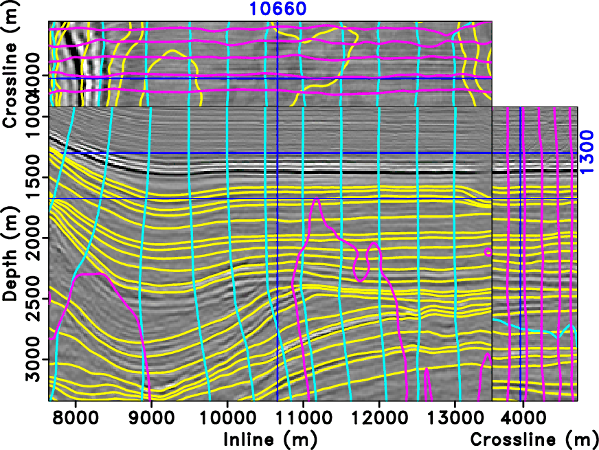
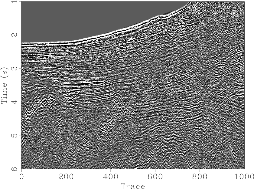
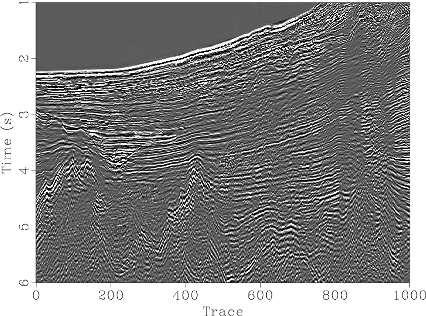
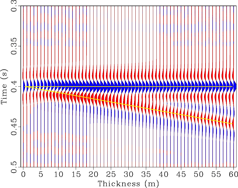
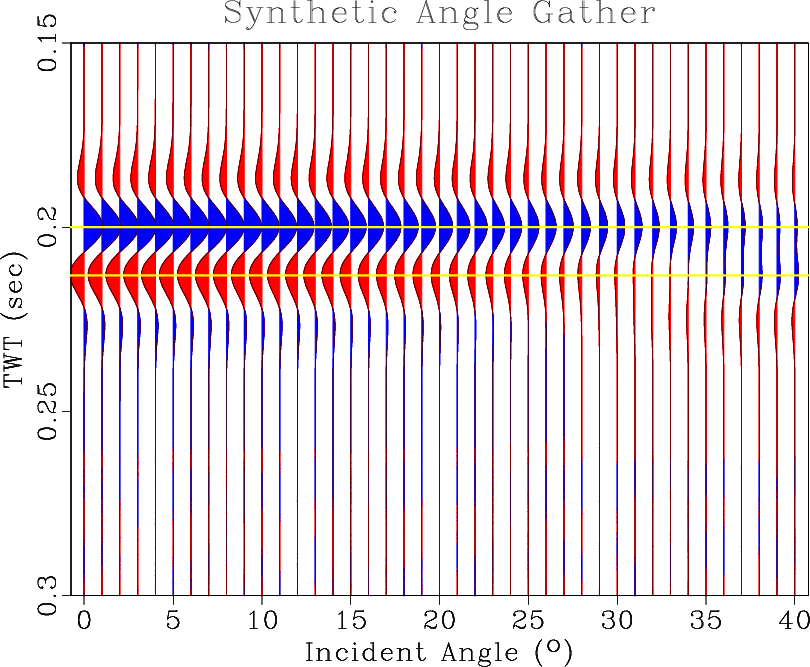
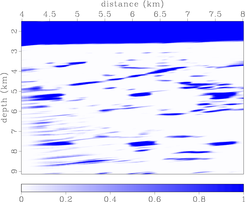
In certain seismic data processing and interpretation tasks, such as spiking deconvolution, tuning analysis, impedance inversion, spectral decomposition, etc., it is commonly assumed that the vertical direction is normal to reflectors. This assumption is false in the case of dipping layers and may therefore lead to inaccurate results. To overcome this limitation, we propose a coordinate system in which geometry follows the shape of each reflector and the vertical direction corresponds to normal reflectivity. We call this coordinate system stratigraphic coordinates. We develop a constructive algorithm that transfers seismic images into the stratigraphic coordinate system. The algorithm consists of two steps. First, local slopes of seismic events are estimated by plane-wave destruction; then structural information is spread along the estimated local slopes, and horizons are picked everywhere in the seismic volume by the predictive-painting algorithm. These picked horizons represent level sets of the first axis of the stratigraphic coordinate system. Next, an upwind finite-difference scheme is used to find the two other axes, which are perpendicular to the first axis, by solving the appropriate gradient equations. After seismic data are transformed into stratigraphic coordinates, seismic horizons should appear flat, and seismic traces should represent the direction normal to the reflectors. Immediate applications of the stratigraphic coordinate system are in seismic image flattening and spectral decomposition. Synthetic and real data examples demonstrate the effectiveness of stratigraphic coordinates.

A new paper is added to the collection of reproducible documents:
Carbonate reservoir characterization using seismic diffraction imaging

Although extremely prolific worldwide, carbonate reservoirs are challenging to characterize using traditional seismic reflection imaging techniques. We use computational experiments with synthetic models to demonstrate the possibility seismic diffraction imaging has of overcoming common obstacles associated with seismic reflection imaging and aiding interpreters of carbonate systems. Diffraction imaging improves the horizontal resolution of individual voids in a karst reservoir model and identification of heterogeneous regions below the resolution of reflections in a reservoir scale model.

A new paper is added to the collection of reproducible documents:
Random noise attenuation using local signal-and-noise orthogonalization

We propose a novel approach to attenuate random noise based on local signal-and-noise orthogonalization. In this approach, we first remove noise using one of the conventional denoising operators, and then apply a weighting operator to the initially denoised section in order to predict the signal-leakage energy and retrieve it from the initial noise section. The weighting operator is obtained by solving a least-squares minimization problem via shaping regularization with a smoothness constraint. Next, the initially denoised section and the retrieved signal are combined to form the final denoised section. The proposed denoising approach corresponds to orthogonalizing the initially denoised signal and noise in a local manner. We evaluate denoising performance by using local similarity. In order to test the orthogonalization property of the estimated signal and noise, we calculate the local similarity map between the denoised signal section and removed noise section. Low values of local similarity indicate a good orthogonalization and thus a good denoising performance. Synthetic and field data examples demonstrate the effectiveness of the proposed approach in applications to noise attenuation for both conventional and simultaneous-source seismic data.

Another old paper is added to the collection of reproducible documents:
Seismic AVO analysis of methane hydrate structures

Marine seismic data from the Blake Outer Ridge offshore Florida show strong “bottom simulating reflections” (BSR) associated with methane hydrate occurence in deep marine sediments. We use a detailed amplitude versus offset (AVO) analysis of these data to explore the validity of models which might explain the origin of the bottom simulating reflector. After careful preprocessing steps, we determine a BSR model which can successfully reproduce the observed AVO responses. The P- and S-velocity behavior predicted by the forward modeling is further investigated by estimating the P- and S-impedance contrasts at all subsurface positions. Our results indicate that the Blake Outer Ridge BSR is compatible with a model of methane hydrate in sediment, overlaying a layer of free methane gas-saturated sediment. The hydrate-bearing sediments seem to be characterized by a high P-wave velocity of approximately 2.5 km/s, an anomalously low S-wave velocity of approximately 0.5 km/s, and a thickness of around 190 meters. The underlaying gas-saturated sediments have a P-wave velocity of 1.6 km/s, an S-wave velocity of 1.1 km/s, and a thickness of approximately 250 meters.