FWI: data mismatch minimization

Next: Nonlinear conjugate gradient method Up: FWI and its GPU Previous: FWI and its GPU

FWI: data mismatch minimization

In the case of constant density, the acoustic wave equation is specified by

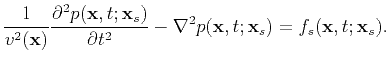$\displaystyle \frac{1}{v^2(\textbf{x})}\frac{\partial^2 p(\textbf{x},t;\textbf{... ...tial t^2}-\nabla^2 p(\textbf{x},t;\textbf{x}_s)=f_s(\textbf{x},t;\textbf{x}_s).$

(1)

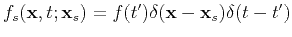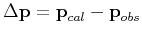where we have set $f_s(\textbf{x},t;\textbf{x}_s)=f(t')\delta(\textbf{x}-\textbf{x}_s)\delta(t-t')$ . According to the above equation, a misfit vector $\Delta \textbf{p}=\textbf{p}_{cal}-\textbf{p}_{obs}$ can be defined by the differences at the receiver positions between the recorded seismic data $\textbf{p}_{obs}$ and the modeled seismic data $\textbf{p}_{cal}=\textbf{f}(\textbf{m})$ for each source-receiver pair of the seismic survey. Here, in the simplest acoustic velocity inversion, $\textbf{f}(\cdot)$ indicates the forward modeling process while $\textbf{m}$ corresponds to the velocity model to be determined. The goal of FWI is to match the data misfit by iteratively updating the velocity model. The objective function taking the least-squares norm of the misfit vector $\Delta \textbf{p}$ is given by

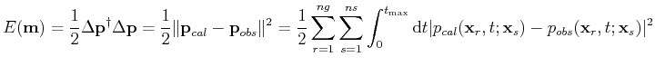$\displaystyle E(\textbf{m})=\frac{1}{2}\Delta \textbf{p}^{\dagger}\Delta \textb... ...cal}(\textbf{x}_r, t;\textbf{x}_s)-p_{obs}(\textbf{x}_r, t;\textbf{x}_s)\vert^2$

(2)

where

and

are the number of sources and geophones, $\dagger$ denotes the adjoint operator (conjugate transpose). The recorded seismic data is only a small subset of the whole wavefield at the locations specified by sources and receivers.

The gradient-based minimization method updates the velocity model according to a descent direction $\textbf{d}_k$ :

$\displaystyle \textbf{m}_{k+1}=\textbf{m}_k+\alpha_k \textbf{d}_k.$

(3)

where

denotes the iteration number. By neglecting the terms higher than the 2nd order, the objective function can be expanded as

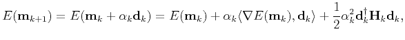$\displaystyle E(\textbf{m}_{k+1})=E(\textbf{m}_k+\alpha_k \textbf{d}_{k})=E(\te... ...}_k\rangle+\frac{1}{2}\alpha_k^2\textbf{d}_k^{\dagger}\textbf{H}_k\textbf{d}_k,$

(4)

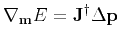
where $\textbf{H}_k$ stands for the Hessian matrix; $\langle\cdot,\cdot\rangle$ denotes inner product. Differentiation of the misfit function $E(\textbf{m}_{k+1})$ with respect to $\alpha_k$ gives

$\displaystyle \alpha_k=-\frac{\langle\textbf{d}_k,\nabla E(\textbf{m}_k)\rangle... ...{cal}\rangle}{\langle\textbf{J}_k\textbf{d}_k,\textbf{J}_k\textbf{d}_k\rangle},$

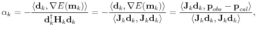(5)

in which we use the approximate Hessian 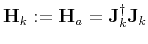$\textbf{H}_k:=\textbf{H}_a=\textbf{J}_k^{\dagger}\textbf{J}_k$ and $\nabla_{\textbf{m}}E=\textbf{J}^{\dagger}\Delta \textbf{p}$ , according to equation (A-7). A detailed derivation of the minimization process is given in Appendix A.

Next: Nonlinear conjugate gradient method Up: FWI and its GPU Previous: FWI and its GPU

2021-08-31