Simulating propagation of separated wave modes in general anisotropic media, Part I: qP-wave propagators

1.3 BP 2007 TTI model

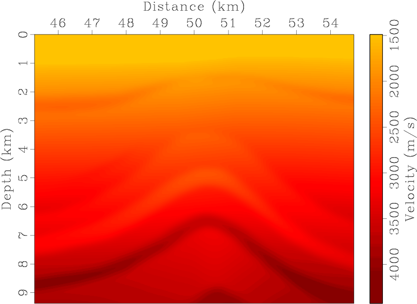
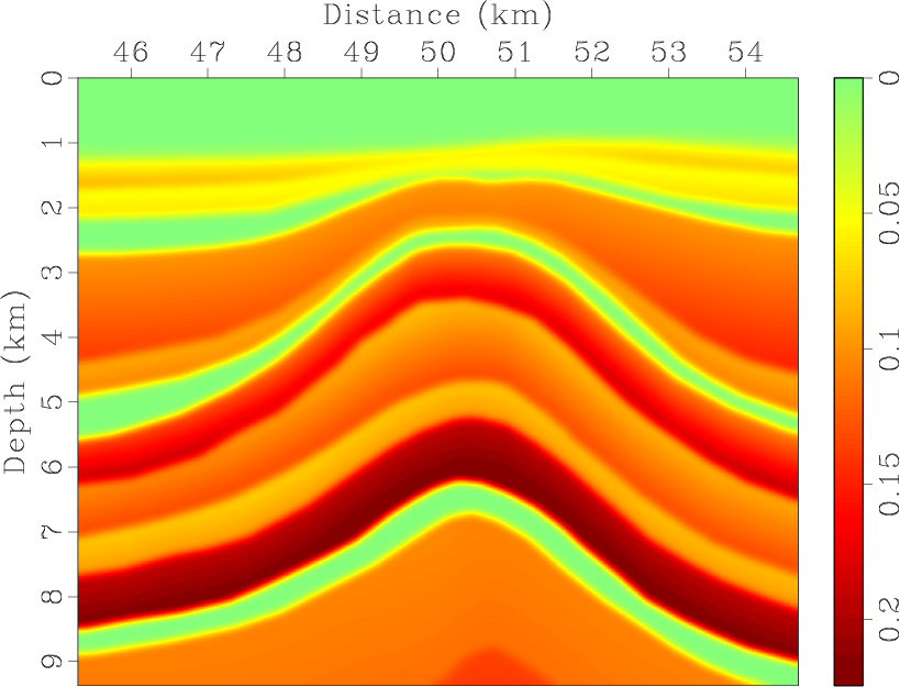
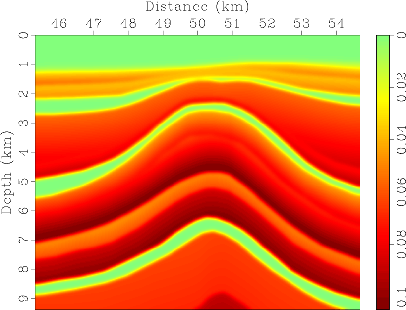
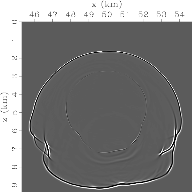
Next we test the approach of simulating propagation of the separated qP-wave mode in a complex TTI model. Figure 7 shows parameters for part of the BP 2D TTI model. The space grid size is 12.5 m and the time step is 1 ms for high-order finite-difference operators. Here the vertical velocities for the qSV-wave are set as half of the qP-wave velocities. Figure 8 displays snapshots of wavefield components at the time of 1.4s synthesized by using original elastic wave equation and pseudo-pure-mode qP-wave equation. The two pictures at the bottom represent the scalar pseudo-pure-mode qP-wave and the separated qP-wave fileds, respectively. The correction appears to remove residual qSV-waves and accurately separate qP-wave data including the converted qS-qP waves from the pseudo-pure-mode wavefields in this complex model.

vp0,epsi,del,the
Figure 7. Partial region of the 2D BP TTI model: (a) vertical qP-wave velocity, Thomsen coefficients (b) $\epsilon$ and (c) $\delta$ , and (d) the tilt angle $\theta$ .

Elasticx,Elasticz,PseudoPurePx,PseudoPurePz,PseudoPureP,PseudoPureSepP
Figure 8. Synthesized elastic wavefields on BP 2007 TTI model using original elastic wave equation and pseudo-pure-mode qP-wave equation respectively: (a) x- and (b) z-components synthesized by original elastic wave equation; (c) x- and (d) z-components synthesized by pseudo-pure-mode qP-wave equation; (e) pseudo-pure-mode scalar qP-wave fields; (f) separated scalar qP-wave fields.

Simulating propagation of separated wave modes in general anisotropic media, Part I: qP-wave propagators