Linear gradient model

Next: Land field data example Up: Examples Previous: Linear sloth model

Linear gradient model

We further test the proposed method with another synthetic model that contains stronger velocity variations in both vertical and horizontal directions. In this model, the exact velocity is given by

$\displaystyle v (z,x) = v_0 + g_z z + g_x x\;,$

(23)

where

, and

. These parameters give 33-50 $\%$ changes in horizontal velocity and a maximum of 60 $\%$ change in vertical velocity. The analytical solutions to time-to-depth conversion in this particular type of model were given by (Li and Fomel, 2015):

$\displaystyle x_0 (z,x)$	$\displaystyle =$	$\displaystyle x + \frac{\sqrt{(v_0+g_x x)^2 + g_x^2 z^2} - (v_0 + g_x x)}{g_x}~,$	(24)
$\displaystyle t_0 (z,x)$	$\displaystyle =$	$\displaystyle \frac{1}{g} \mathrm{arccosh} \left[ \frac{g^2 \left( \sqrt{(v_0+g_x x)^2 + g_x^2 z^2} + g_z z \right) - v g_z^2}{v g_x^2} \right]~,$	(25)

where $g = \sqrt{g_z^2 + g_x^2}$ denotes the magnitude of the total gradient. It follows from equations 24 and 25 that $\vert\nabla x_0\vert=1$ , $\vert\nabla t_0\vert=1/v$ , and $\nabla x_0 \cdot \nabla t_0 = 1$ , which indicate that the geometrical spreading of image rays in this model is equal to one and the Dix velocity is equal to the interval velocity expressed in the time-domain coordinates

and

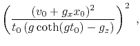
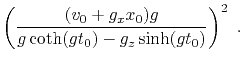
(equation 3). Nonetheless, the image rays still bend laterally because $g_x \ne 0$ and will lead to distorted time-domain coordinates. The migration velocity squared

and its Dix-inverted counterpart

can also be derived analytically and are given by (Li and Fomel, 2015):

$\displaystyle w_m (t_0,x_0)$	$\displaystyle =$	$\displaystyle \left(\frac{(v_0 + g_x x_0)^2}{t_0 \left( g \coth (g t_0) - g_z \right)} \right)^2~,$	(26)
$\displaystyle w_d (t_0,x_0)$	$\displaystyle =$	$\displaystyle \left(\frac{(v_0 + g_x x_0) g}{g \coth (g t_0) - g_z \sinh (g t_0)}\right)^2~.$	(27)

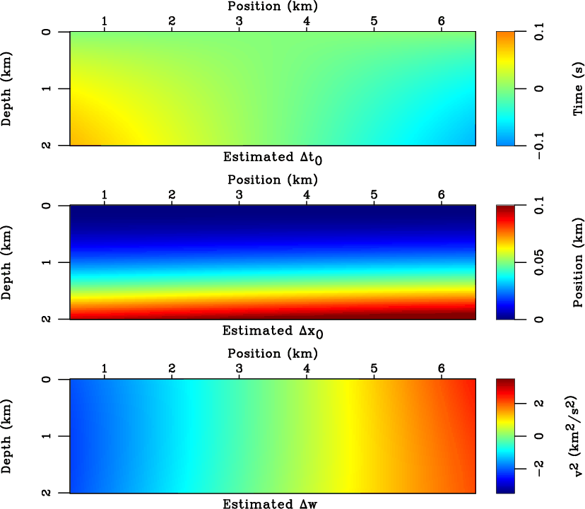
Figure 7 shows the true interval velocity of the model (equation 23), and the analytical and overlaid by the contours that show image rays and propagating image wavefront. Figure 8 shows other inputs for the proposed conversion method. Again, we arbitrarily choose the reference background to be the central trace of the reference $w_{dr}(x,z)$ . Figure 9 shows the final estimated values of the three quantities-- $\Delta x_0$ , $\Delta t_0$ , and $\Delta w$ . Their corresponding errors are shown in Figure 10 suggesting a reasonable accuracy of the proposed method when the true velocity is close to the reference $w_{r}(z)$ in the middle of the model. Higher errors are observed as the velocity difference becomes larger closer to the side and bottom edges.


model-grad Figure 7. The true velocity squared (top) of the linear gradient model (equation 23). Analytical (middle) is overlaid by image rays. Analytical (bottom) is overlaid by contours showing propagating image wavefront.


input-grad Figure 8. Inputs of the proposed time-to-depth conversion for the linear gradient model. The last input (not shown here) is taken to be the central trace of $w_{dr}(x,z)$ (top) in this case.


estcompare-grad Figure 9. The estimated values of $\Delta x_0$ , $\Delta t_0$ , $\Delta w$ in the linear gradient model (equation 23).


errcompare-grad Figure 10. The errors of the estimated values of $\Delta x_0$ , $\Delta t_0$ , $\Delta w$ in comparison with the true values in the linear gradient model (equation 23). The errors are small for all estimated parameters except in the vicinity of the side and bottom edges of the model, which could be attributed to the growing difference between the true value of in that region and the reference in the middle of the model.

errcompare-grad
Figure 10. The errors of the estimated values of $\Delta x_0$ , $\Delta t_0$ , $\Delta w$ in comparison with the true values in the linear gradient model (equation 23). The errors are small for all estimated parameters except in the vicinity of the side and bottom edges of the model, which could be attributed to the growing difference between the true value of

in that region and the reference

in the middle of the model.

Next: Land field data example Up: Examples Previous: Linear sloth model

2018-11-16