 |
 |
 |
 | Fast time-to-depth conversion and interval velocity estimation in the case of weak lateral variations |  |
![[pdf]](icons/pdf.png) |
Next: Taking weak lateral variations
Up: Sripanich & Fomel: Time
Previous: Introduction
The time-domain coordinates  used in time migration are related to the Cartesian depth coordinates
  through the knowledge of image rays (Figure 2), which have orthogonal slowness vector to the surface (Hubral, 1977). For each subsurface location
, an image ray travels through the medium and emerges at
through the knowledge of image rays (Figure 2), which have orthogonal slowness vector to the surface (Hubral, 1977). For each subsurface location
, an image ray travels through the medium and emerges at  with traveltime
  . The forward maps
  and
and  can be obtained with the knowledge of the interval velocity
  . We can also define the inverse maps
 and
and
 for the time-to-depth conversion process. Similar description of coordinates relation also holds in 3D.

|
|---|
imageray
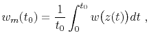
Figure 2. The relationship between time-domain coordinates and the Cartesian depth coordinates. An example image ray with slowness vector normal to the surface travels from the source  into the subsurface. Every point along this ray is mapped to the same distance location
in the time coordinates with different corresponding traveltime
into the subsurface. Every point along this ray is mapped to the same distance location
in the time coordinates with different corresponding traveltime  .
.
|
|---|
![[png]](icons/viewmag.png)
|
|---|
In time domain, one operates with the time-migration velocity
 estimated from migration velocity analysis (Yilmaz, 2001; Fomel, 2003a,b). In a laterally homogeneous medium,
  corresponds theoretically to the RMS velocity:
 |
(1) |
where we denote  throughout the text. The inverse process to recover interval velocity
  can be done through the Dix inversion (Dix, 1955):
 |
(2) |
where the subscript  is used to denote the Dix-inverted parameter. A simple conversion from
  to
to  reduces then to a straightforward integration over time to obtain a
  map.
map.
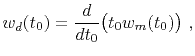
On the other hand, in the case of laterally heterogeneous media, Cameron et al. (2007) proved that the Dix-inverted velocity can be related to the true interval velocity by the geometrical spreading
 of the image rays traced telescopically from the surface as follows:
 |
(3) |
where the geometrical spreading  satisfies,
 |
(4) |
Combining equations 3 and 4 gives
 |
(5) |
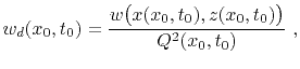
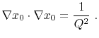
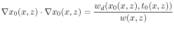
To solve for the interval velocity, two additional equations are needed (Cameron et al., 2007; Li and Fomel, 2015):
Equation 6 indicates that  is constant along each image ray, and equation 7 denotes the eikonal equation of image ray propagation. Equations 5-7 amount to a system of PDEs that can be solved for the interval velocity
as well as the maps
and
needed for the time-to-depth conversion process.
is constant along each image ray, and equation 7 denotes the eikonal equation of image ray propagation. Equations 5-7 amount to a system of PDEs that can be solved for the interval velocity
as well as the maps
and
needed for the time-to-depth conversion process.
Subsections
|
|
|
|
| Fast time-to-depth conversion and interval velocity estimation in the case of weak lateral variations | |
|
Next: Taking weak lateral variations
Up: Sripanich & Fomel: Time
Previous: Introduction
2018-11-16
