Lowrank seismic wave extrapolation on a staggered grid

2D examples of a two-layer model

To test the performance of the proposed methods with a rough velocity model, we use a two-layer model with high velocity and density contrasts. The model is defined on a $501 \times 501$ grid, with $\Delta x=\Delta z=10 m$ and $\Delta t=1.5ms$ . Velocities of the upper and lower layers are $1.3 km/s$ and $3.2 km/s$ . The densities of upper and lower layers are $1.7 g/cm^3$ and $2.7 g/cm^3$ respectively. A point source of a Ricker-wavelet with dominant frequency of 20 Hz is located in the center of the model at a depth of $0.2 km$ .The maximum frequency ($f_{max}$ ) is around $60Hz$ . Following Song et al. (2013), we still use the CFL number $\alpha$ to specify the stability and define dispersion factor as $\beta=v_{min}/(f_{max}\Delta x)$ to indicate the sample points per wavelength, where $v_{min}$ is the minimum velocity of the model. For modeling with above parameters, $\alpha=0.32$ and $\beta=2.2$ .

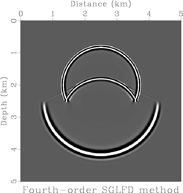
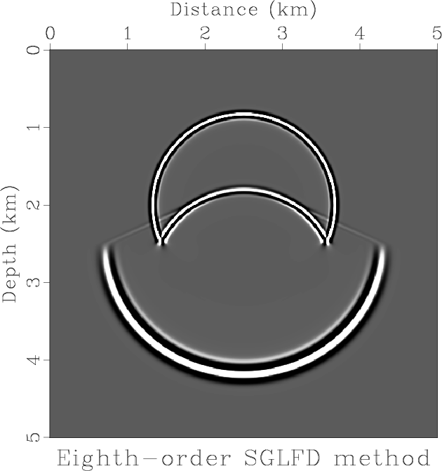
Figure 12 shows a wavefield snapshot generated by lowrank FD with a time interval equal to $2 ms$ . At this time interval, the SGFD method becomes unstable.

lfd4snap2,lfd8snap2
Figure 12. Wavefield snapshot in a two-layer model with variable density and velocity using (a) 4th order SGLFD method and (b) 8th order SGLFD method.

Lowrank seismic wave extrapolation on a staggered grid