Seislet transform and seislet frame

2-D data analysis with 1-D seislet frame

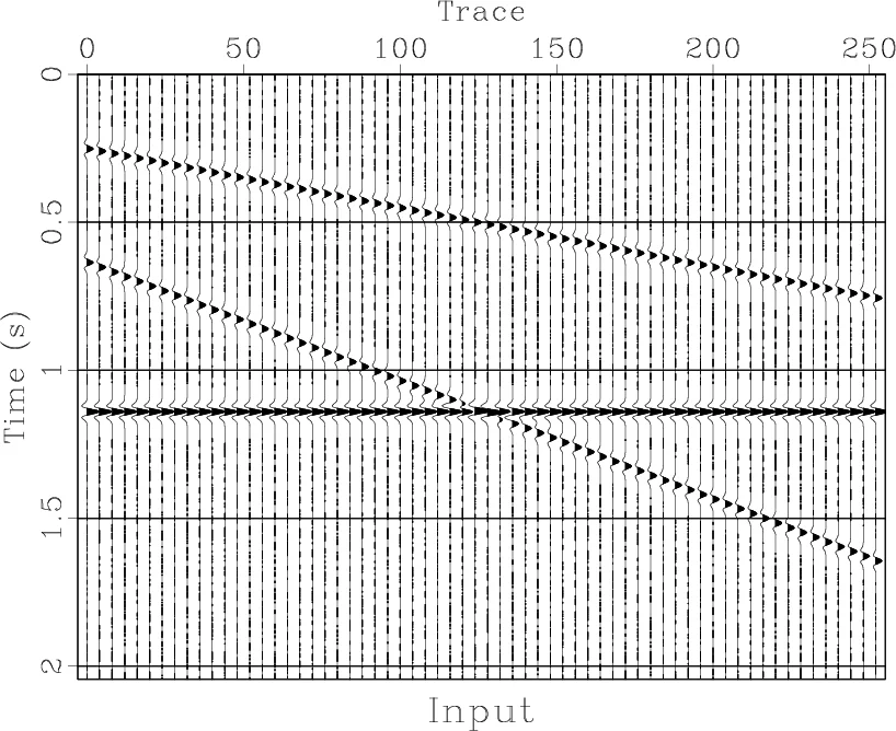
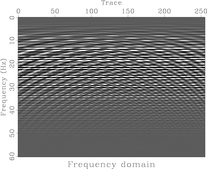
To analyze 2-D data, one can apply 1-D seislet frame in the distance direction after the Fourier transform in time (the - domain). In this case, different frame frequencies correspond to different plane-wave slopes (Canales, 1984). We use a simple plane-wave synthetic model to verify this observation (Figure 15a). The - plane is shown in Figure 15b. We find a prediction-error-filter (PEF) in each frequency slice and detect its roots to select appropriate spatial frequencies. We use Burg's algorithm for PEF estimation (Claerbout, 1976; Burg, 1975) and an eigenvalue-based algorithm for root finding (Edelman and Murakami, 1995). The seislet coefficients and the corresponding recovered plane-wave components are shown in Figure 16. Similarly to the 1-D example, information from different plane-waves gets strongly compressed in the transform domain.

plane,fft Figure 15. Synthetic plane-wave data (a) and corresponding Fourier transform along the time direction (b).

plane1,plane2,plane3 Figure 16. Seislet coefficients (left) and corresponding recovered plane-wave components (right) for three different parts of the 1-D seislet frame in the - domain.

Seislet transform and seislet frame