Non-stationary Prony method

Equation 27 can be written as a matrix form:

$\displaystyle \sum_{m=1}^{M}\mathbf{\hat{a}}_m(t)\mathbf{x}_m(t) \approx \mathbf{d}(t),$

(36)

where $\mathbf{d}(t) = \mathbf{x}(t)$ , $\mathbf{x}_m(t) = \mathbf{x}(t-m\Delta t)$ is the time shift of the input signal $\mathbf{x}(t)$ and $\mathbf{\hat{a}}_m(t)$ is the time-dependant coefficients. We solve the under-determined linear system by using the shaping regularization method. The solution is the form below:

$\displaystyle \mathbf{a = F^{-1}\eta},$

(37)

where $\mathbf{a}$ is a vector of $\hat{a}(t)$ , the elements of vector $\mathbf{\eta}$ is:

$\displaystyle \mathbf{\eta}_i(t) = \mathbf{S}\left[\mathbf{x}_i^*(t)\mathbf{d}(t)\right],$

(38)

the elements of the matrix $\mathbf{F}$ is:

$\displaystyle \mathbf{F}_{ij}= \sigma^2 \mathbf{\delta}_{ij} + S[\mathbf{x}_i^*(t)\mathbf{x}_j(t) - \sigma^2 \mathbf{\delta}_{ij}]$

(39)

where $\sigma$ is the regularization parameter, $\mathbf{S}$ is a shaping operator, and $\mathbf{x}_i^*(t)$ stands for the complex conjugate of $\mathbf{x}_i(t)$ . We can use the conjugate gradient method to find the solution of the linear system. The NPM (Fomel, 2013) can be summarized as follows:

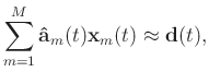
$\begin{algorithm}{Algorithm 2: non-stationary Prony method}{} \text{Find time d... ...m=1}^M \hat{A}_m[n]e^{j\hat{\phi}_m[n]}=\sum_{m=1}^M\hat{c}_m[n] \end{algorithm}$

After we decompose the input signal into narrow-band components, we compute the time-frequency distribution of the input signal using the Hilbert transform of the intrinsic mode functions.

2020-07-18