Next: CONCLUSIONS Up: Fomel, Ying, & Song: Previous: LOWRANK APPROXIMATION

EXAMPLES

We start with a simple 1-D example. The 1-D velocity model contains a linear increase in velocity, from 1 km/s to 2.275 km/s. The extrapolation matrix, $2 (\cos\left[V(x) \vert k\vert \Delta t\right]-1)$ , or pseudo-Laplacian in the terminology of Etgen and Brandsberg-Dahl (2009), for the time step $\Delta t=0.001$ s is plotted in Figure 1a. Its lowrank approximation is shown in Figure 1b and corresponds to . The locations selected by the algorithm correspond to velocities of 1.59 and 2.275 km/s. The wavenumbers selected by the algorithm correspond to the Nyquist frequency and 0.7 of the Nyquist frequency. The approximation error is shown in Figure 1c. The relative error does not exceed 0.34%. Such a small approximation error results in accurate wave extrapolation, which is illustrated in Figure 2. The extrapolated wavefield shows a negligible error in wave amplitudes, as demonstrated in Figure 2c.


prop,prod,proderr Figure 1. Wave extrapolation matrix for 1-D wave propagation with linearly increasing velocity (a), its lowrank approximation (b), and Approximation error (c).


wave2,awave2,waverr Figure 2. (a) 1-D wave extrapolation using the exact extrapolation symbol. (b) 1-D wave extrapolation using lowrank approximation. (c) Difference between (a) and (b), with the scale amplified 10 times compared to (a) and (b).


wavefd,wave Figure 3. Wavefield snapshot in a smooth velocity model computed using (a) fourth-order finite-difference method and (b) lowrank approximation. The velocity model is . The wave source is a point-source Ricker wavelet, located in the middle of the model. The finite-difference result exhibits dispersion artifacts while the result of the lowrank approximation, similarly to that of the FFD method, is dispersion-free.

wavefd,wave
Figure 3. Wavefield snapshot in a smooth velocity model computed using (a) fourth-order finite-difference method and (b) lowrank approximation. The velocity model is

. The wave source is a point-source Ricker wavelet, located in the middle of the model. The finite-difference result exhibits dispersion artifacts while the result of the lowrank approximation, similarly to that of the FFD method, is dispersion-free.


slicefd,slice Figure 4. Horizontal slices through wavefield snapshots in Figure 3

Our next example (Figures 3 and 4) corresponds to wave extrapolation in a 2-D smoothly variable isotropic velocity field. As shown by Song and Fomel (2011), the classic finite-difference method (second-order in time, fourth-order in space) tends to exhibit dispersion artifacts with the chosen model size and extrapolation step, while spectral methods exhibit high accuracy. As yet another spectral method, the lowrank approximation is highly accurate. The wavefield snapshot, shown in Figures 3b and 4b, is free from dispersion artifacts and demonstrates high accuracy. The approximation rank decomposition in this case is , with the expected error of less than $10^{-4}$ . In our implementation, the CPU time for finding the lowrank approximation was 2.45 s, the single-processor CPU time for extrapolation for 2500 time steps was 101.88 s or 2.2 times slower than the corresponding time for the finite-difference extrapolation (46.11 s).


fwavefd,fwave Figure 5. Wavefield snapshot in a simple two-layer velocity model using (a) fourth-order finite-difference method and (b) lowrank approximation. The upper-layer velocity is 1500 m/s, and the bottom-layer velocity is 4500 m/s. The finite-difference result exhibits clearly visible dispersion artifacts while the result of the lowrank approximation is dispersion-free.

To show that the same effect takes place in case of rough velocity model, we use first a simple two-layer velocity model, similar to the one used by Fowler et al. (2010). The difference between a dispersion-infested result of the classic finite-difference method (second-order in time, fourth-order in space) and a dispersion-free result of the lowrank approximation is clearly visible in Figure 5. The time step was 2 ms, which corresponded to the approximation rank of 3. In our implementation, the CPU time for finding the lowrank approximation was 2.69 s, the single-processor CPU time for extrapolation for 601 time steps was 19.76 s or 2.48 times slower than the corresponding time for the finite-difference extrapolation (7.97 s). At larger time steps, the finite-difference method in this model becomes unstable, while the lowrank method remains stable but requires a higher rank.


sub Figure 6. Portion of BP-2004 synthetic isotropic velocity model.


snap Figure 7. Wavefield snapshot for the velocity model shown in Figure 6.

Next, we move to isotropic wave extrapolation in a complex 2-D velocity field. Figure 6 shows a portion of the BP velocity model (Billette and Brandsberg-Dahl, 2005), containing a salt body. The wavefield snapshot (shown in Figure 7) confirms the ability of our method to handle complex models and sharp velocity variations. The lowrank decomposition in this case corresponds to , with the expected error of less than $10^{-7}$ . Increasing the time step size $\Delta t$ does not break the algorithm but increases the rank of the approximation and correspondingly the number of the required Fourier transforms. For example, increasing $\Delta t$ from 1 ms to 5 ms leads to .


salt Figure 8. SEG/EAGE 3-D salt model.


wave3 Figure 9. Snapshot of a point-source wavefield propagating in the SEG/EAGE 3-D salt model.

Our next example is isotropic wave extrapolation in a 3-D complex velocity field: the SEG/EAGE salt model (Aminzadeh et al., 1997) shown in Figure 8. A dispersion-free wavefield snapshot is shown in Figure 9. The lowrank decomposition used , with the expected error of $10^{-5}$ .


vpend2,vxend2,etaend2,thetaend2 Figure 10. Portion of BP-2007 anisotropic benchmark model. (a) Velocity along the axis of symmetry. (b) Velocity perpendicular to the axis of symmetry. (c) Anellipticity parameter $\eta$ . (d) Tilt of the symmetry axis.


snap4299 Figure 11. Wavefield snapshot for the velocity model shown in Figure 10.

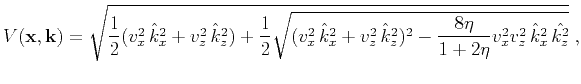
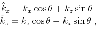
Finally, we illustrate wave propagation in a complex anisotropic model. The model is a 2007 anisotropic benchmark dataset from BP. It exhibits a strong TTI (tilted transverse isotropy) with a variable tilt of the symmetry axis (Figure 10). A wavefield snapshot is shown in Figure . Because of the complexity of the wave propagation patterns, the lowrank decomposition took in this case and required 10 FFTs per time step. In a TTI medium, the phase velocity $V(\mathbf{x},\k )$ from equation (10) can be expressed with the help of the acoustic approximation (Fomel, 2004; Alkhalifah, 1998 2000)

$\displaystyle V(\mathbf{x},\k ) = \sqrt{\frac{1}{2}(v_x^2 \hat{k}_x^2+v_z^2 \... ... \hat{k}_z^2)^2-\frac{8\eta}{1+2\eta}v_x^2v_z^2 \hat{k}_x^2 \hat{k_z^2}}}\;,$

(15)

where

is the P-wave phase velocity in the symmetry plane,

is the P-wave phase velocity in the direction normal to the symmetry plane, $\eta$ is the anellipticity parameter (Alkhalifah and Tsvankin, 1995), and $\hat{k}_x$ and $\hat{k}_z$ stand for the wavenumbers evaluated in a rotated coordinate system aligned with the symmetry axis:

$\begin{displaymath}\begin{array}{*{20}c} \hat{k}_x=k_x\cos{\theta}+k_z\sin{\theta}\;\ \hat{k}_z=k_z\cos{\theta}-k_x\sin{\theta}\;,\ \end{array}\end{displaymath}$

(16)

where $\theta$ is the tilt angle measured with respect to horizontal.

Next: CONCLUSIONS Up: Fomel, Ying, & Song: Previous: LOWRANK APPROXIMATION

2013-08-31