Velocity continuation by spectral methods

Fourier approach

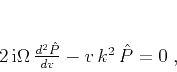
Introducing the change of variable $\sigma = t^2$, we can transform equation (1) to the form

$$2 \frac{\partial^2 P}{\partial v \partial \sigma} + v \frac{\partial^2 P}{\partial x^2} = 0\;,$$ (5)

whose coefficients don't depend on the time variables. Double Fourier transform in $\sigma$ and $x$ further simplifies equation (5) to the ordinary differential equation

$$2 i\Omega \frac{d^2 \hat{P}}{d v} - v k^2 \hat{P} = 0\;,$$ (6)

where the frequency $\Omega$ corresponds to the time coordinate $\sigma$, and $k$ is the wavenumber in $x$. Equation (6) has an explicit analytical solution

$$\hat{P} (k,\Omega,v) = \hat{P}_0 (k,\Omega) e^{\frac{i k^2(v_0^2-v^2)}{4\Omega}}\;,$$ (7)

which defines a very simple algorithm for the numerical velocity continuation. The algorithms consists of the following steps:

1. Transform the input from a regular grid in $t$ to a regular grid in $\sigma$.
2. Apply FFT in $x$ and $\sigma$.
3. Multiply by the all-pass phase-shift filter $e^{\frac{i k^2(v_0^2-v^2)}{4\Omega}}$.
4. Inverse FFT in $x$ and $\sigma$.
5. Inverse transform to a regular grid in $t$.

t2
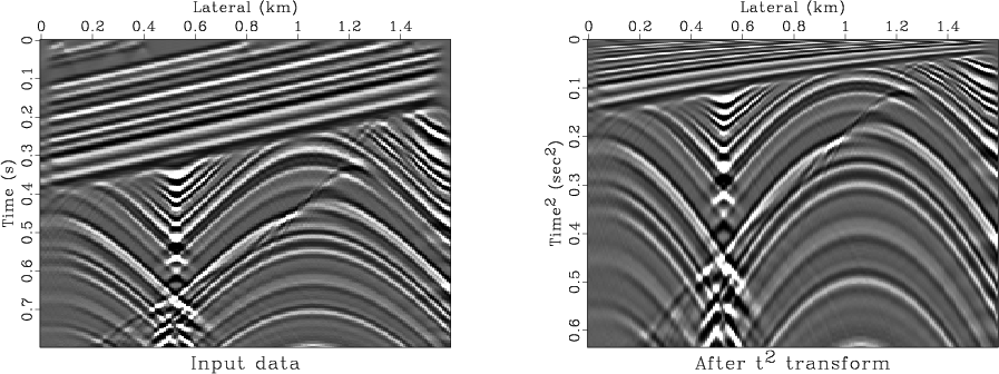
Figure 2. Synthetic seismic data before (left) and after (right) transformation to the $\sigma$ grid.

Figure 2 shows a simple synthetic model of seismic reflection data from (Claerbout, 1995) before and after transforming the grid, regularly spaced in $t$, to a grid, regular in $\sigma$. The left plot of Figure 3 shows the Fourier transform of the data. Except for the nearly vertical event, which corresponds to a stack of parallel layers in the shallow part of the data, the data frequency range is contained near the origin in the $\Omega-k$ space. The right plot of Figure 3 shows the phase-shift filter for continuation from zero imaging velocity (which corresponds to unprocessed data) to the velocity of 1 km/sec. The rapidly oscillating part (small frequencies and large wavenumbers) is exactly in the place, where the data spectrum is zero and corresponds to physically impossible reflection events.

t2-fft
Figure 3. Left: the real part of the data Fourier transform. Right: the real part of the velocity continuation operator (continuation from 0 to 1 km/s) in the Fourier domain.

Algorithm (7) is very attractive from the practical point of view because of its efficiency (based on the FFT algorithm). The operations count is roughly the same as in Stolt migration (4): two forward and inverse FFTs and forward and inverse grid transform with interpolation (one complex-number transform in the case of Stolt migration). Algorithm (7) can be even more efficient than Stolt method because of the simpler structure of the innermost loop. However, its practical implementation faces two difficult problems: artifacts of the $t^2$ grid transform and wraparound artifacts

Velocity continuation by spectral methods