Spectral factorization revisited

A comparison with the Wilson-Burg method

For reasons of symmetry, we can take Newton's relation from Table 3

$$X_{n+1} =\frac{S+X_n \bar X_n}{2\bar X_n}$$

and convert it to

$$\frac{X_{n+1}}{2 X_n} = \frac{S+X_n \bar X_n}{(2 X_n) (2\bar X_n)}.$$

We can then consider a symmetrical relation where on the left side we insert the anticausal part of the spectrum, and obtain

$$\frac{\bar X_{n+1}}{2 \bar X_n} = \frac{S+X_n \bar X_n}{(2 X_n) (2\bar X_n)}.$$

Finally, we can sum the preceding two equations and get

$$\fbox{$ \displaystyle \frac{X_{n+1}}{2 X_n} + \frac{\bar X_{n... ...\frac{2S+ X_n \bar X_n + \bar X_n X_n}{(2 X_n) (2\bar X_n)} $}$$ (9)

which can easily be shown to be equivalent to the Wilson-Burg relation

$$\frac{X_{n+1}}{X_n} + \frac{\bar X_{n+1}}{\bar X_n} = 1 + \frac{S}{ X_n \bar X_n}$$ (10)

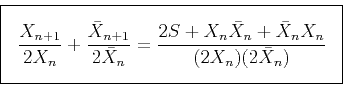
In an analogous way, we can take the general relation from Table 3

$$X_{n+1} =\frac{S+X_n \bar G}{\bar X_n+\bar G}$$

and convert it to

$$\frac{X_{n+1}}{X_n + G} = \frac{S+X_n \bar G}{(X_n + G) (\bar X_n + \bar G)}$$

We can then consider a symmetrical relation where on the left side we insert the anticausal part of the spectrum, and obtain

$$\frac{\bar X_{n+1}}{\bar X_n + \bar G} = \frac{S+\bar X_n G}{(X_n + G) (\bar X_n + \bar G)}$$

Finally, we can sum the preceding two equations and get

$$\fbox{$ \displaystyle \frac{X_{n+1}}{X_n + G} + \frac{\bar X... ...{2S+X_n \bar G + \bar X_n G}{(X_n + G) (\bar X_n + \bar G)} $}$$ (11)

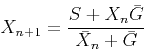
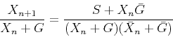
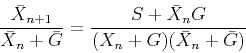
Equation (11) represents our general formula for spectral factorization. If we consider the particular case when $G$ is $X_n$, we obtain equation (10), which we have shown to be equivalent to the Wilson-Burg formula.

From the computational standpoint, our equation is more expensive than the Wilson-Burg because it requires two more convolutions on the numerator of the right-hand side. However, our equation offers more flexibility in the convergence rate. If we try to achieve a quick convergence, we can take $G$ to be $X_n$ and get the Wilson-Burg equation. On the other hand, if we worry about the stability, especially when some of the roots of the auto-correlation function are close to the unit circle, and we fear losing the minimum-phase property of the factors, we can take $G$ to be some damping function, more tolerant of numerical errors.

Moreover, by using the Equation (11), we can achieve fast convergence in cases when the auto-correlations we are factorizing have a very similar form, for example, in nonstationary filtering. In such cases, the solution at the preceding step can be used as the $G$ function in the new factorization. Since $G$ is already very close to the solution, the convergence is likely to occur quite fast.

Spectral factorization revisited