|
|
|
|
Fast Streaming Local Time-frequency Transform for Nonstationary Seismic Data Processing |
Next: Applications Up: Theory Previous: Streaming Local Time-frequency Transform
|
|
|
|
Fast Streaming Local Time-frequency Transform for Nonstationary Seismic Data Processing |
The key different between S-transform and STFT is that S-transform
employs a frequency-varying Gaussian taper, which provides
 spectrum with variable
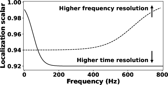
localization. Considering that the localization scalar
spectrum with variable
localization. Considering that the localization scalar
 controls the
localization of SLTFT, we design the new
localization scalar varying over frequency
controls the
localization of SLTFT, we design the new
localization scalar varying over frequency
 |
(21) |
 is the frequency. Increment of the localization scalar
enhances the time localization of the spectrum, albeit at the cost of
the reduced frequency localization, and vice versa. This inverse
relationship allows us to adjust the balance between time and
frequency localization according to specific requirements.
is the frequency. Increment of the localization scalar
enhances the time localization of the spectrum, albeit at the cost of
the reduced frequency localization, and vice versa. This inverse
relationship allows us to adjust the balance between time and
frequency localization according to specific requirements.
We use two synthetic nonstationary models to to illustrate the
time-frequency characterization of the proposed method. The first
model (refered to as signal 1) comprises two hyperbolic signals
 ,
,  and Gaussian noise, where
![\begin{empheq}[left={\empheqlbrace}]{align}
s_1(t) &= \cos\left[{
2\pi\left( {...
...s\left[{
2\pi\left( {-1.5t+\frac{1.25}{0.78-t}} \right)
}\right].
\end{empheq}](img67.png)
The signal 1 with a time interval of 0.5 ms contains 2000 samples
between each sample. We windowed the periodic signals by a
length-fixed cosine taper. The first signal has a time
duration ranging from 0.1 to 0.7 seconds, while the second signal
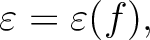
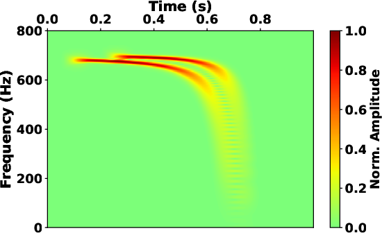
spans from 0.25 to 0.75 seconds. The S-transform provides a
variable
 - localization (see Fig.4a) that allows
the spectrum to exhibit enhanced frequency resolution at lower
frequencies and superior time localization at higher
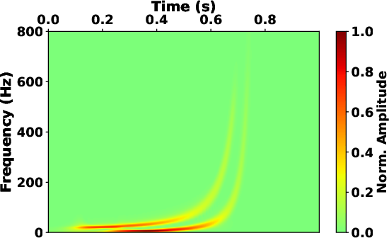
frequencies. Fig.4c shows the spectrum calculated from the
STFT with fixed window length. It is noted that the spectrum exhibits
improved frequency localization at lower frequencies. However, this
enhancement comes at the expense of reduced time localization around
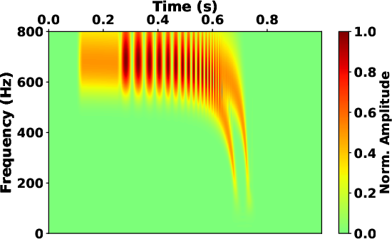
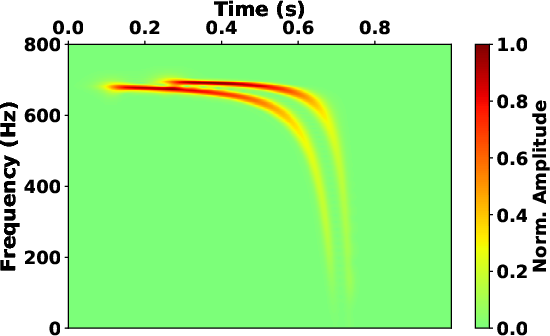
higher frequencies. Therefore, we can apply the frequency-varying
localization scalers (see Fig.4g) to the SLTFT, and the
result (see Fig.4e)
provides a reasonable time-frequency spectrum similar to that of the
S-transform.
- localization (see Fig.4a) that allows
the spectrum to exhibit enhanced frequency resolution at lower
frequencies and superior time localization at higher
frequencies. Fig.4c shows the spectrum calculated from the
STFT with fixed window length. It is noted that the spectrum exhibits
improved frequency localization at lower frequencies. However, this
enhancement comes at the expense of reduced time localization around
higher frequencies. Therefore, we can apply the frequency-varying
localization scalers (see Fig.4g) to the SLTFT, and the
result (see Fig.4e)
provides a reasonable time-frequency spectrum similar to that of the
S-transform.
We selected two different hyperbolic signals  ,
,  in
replace those in the second model (refered to as signal 2) to further
test the SLTFT, where
in
replace those in the second model (refered to as signal 2) to further
test the SLTFT, where
![\begin{empheq}[left={\empheqlbrace}]{align}
s_3(t) &= \cos\left[{
2\pi\left( {...
...os\left[{
2\pi\left( {700t-\frac{1.25}{0.78-t}} \right)
}\right].
\end{empheq}](img71.png)
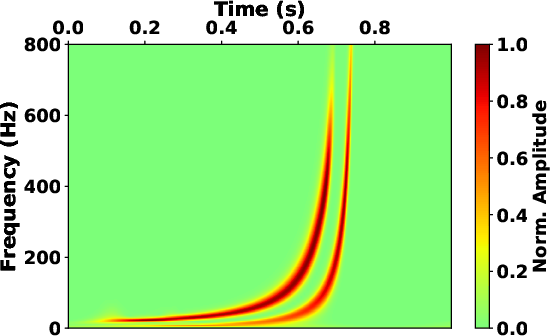
In this case, the S-transform encounters difficulties in producing an
accurate spectrum shown in Fig.4b, which displays
significant aliasing since its high time resolution leads to
diminished frequency localization at higher frequencies. This
observation shows that the variable time-frequency localization
inherent in the S-transform introduces a trade-off between the
representation of low and high frequency components. For comparison,
the STFT with constant window length is hard to achieve a balance
between time and frequency localization. As illustrated in
Fig.4d, the spectrum obtained by the SLTFT with
constant localization scaler exhibits better frequency localization
(around higher frequencies), but comes at the expense of diminished
time localization (at lower frequencies). Fig.4g
shows the frequency-varying localization scalers applied in this case,
which has a trend opposite to that of signal 1. The flexible
frequency-varying parameters lead to a resonable spectrum obtained by
the proposed SLTFT (see Fig.4f).
|
|---|
|
st,st1,stft,stft1,sltft,sltft1,epss
Figure 4. The time-frequency map of synthetic signal 1 obtained by (a) S-transform, (c) STFT with fixed window length and (e) SLTFT with frequency-varying localization scalers. The time-frequency map of synthetic signal 2 obtained by (b) S-transform, (d) STFT with fixed window length and (f) SLTFT with frequency-varying localization scalers. (g) The frequency-varying localization scalers of SLTFT used in Fig.4e (solid line) and Fig.4f (dash line). |
|
|
The above examples show the adaptive and flexible frequency sampling of SLTFT in signal analysis, which provides an adjustable time-frequency representation. Next, we use several field datasets to show its performance in seismic data processing tasks.
|
|
|
|
Fast Streaming Local Time-frequency Transform for Nonstationary Seismic Data Processing |