Streaming Local Time-frequency Transform

The discrete Fourier transform is a vital tool for signal analysis and processing. Given a casual discrete signal $s[n]$ with a fixed length of $N$, its Fourier series can be derived by the inner product of the signal with a family of sines and cosines

$$C[k] = \frac{1}{N}\left< s[n],\psi_k[n] \right> = \frac{1}{N}\sum_{n=0}^{N-1} s[n]e^{-\text{j}2\pi k\Delta f (n/N)},$$ (1)

where $\Delta f$ is the frequency interval, $k$ and $n$ are the discrete frequency index and time index, respectively. $C[k]$ are the Fourier coefficients, $\psi_k[n] = \exp\left[-\text{j}2\pi k\Delta f (n/N)\right]$ are the complex-value bases, and $[\cdot]$ stands for the index of a discrete sequence. The signal can be expressed by the inverse form of equation 1, which is written as

$$s[n] = \left< C[k] ,\psi^*_k[n] \right> = \sum_{k=0}^{N-1} C[k]e^{\text{j}2\pi k\Delta f (n/N)},$$ (2)

where $\psi^*_k[n]$ is the complex conjugate of $\psi_k[n]$. We can rewrite the equation 2 in a prediction-error regression form as

$$e[n] = s[n] - \sum_{k=0}^{N-1} C[k] \psi^*_k[n],$$ (3)

where $e[n]$ is the prediction error. Then we can apply the nonstationary regression (Fomel, 2009) to the Fourier series regression in equation 3, which allows the coefficients $C[k]$ to vary over time coordinate $n$. The error turns into (Fomel, 2009)

$$e[n] = s[n] - \sum_{k=0}^{N-1} C[k,n] \psi^*_k[n].$$ (4)

The nonstationary coefficients $C[k,n]$ can be obtained by solving the least-squares minimization problem(Liu and Fomel, 2013):

$$\min_{C}\,\left\Vert s[n]-\sum_{k=0}^{N-1} C[k,n] \psi_k^{*}[n]\right\Vert_2^2.$$ (5)

The nonstationary regression makes the minimization of equation 5 become ill-posed, and a reasonable solution is to include additional constraints. Classical regularization methods, such as Tikhonov regularization (Tikhonov, 1963) and shaping regularization (Liu and Fomel, 2013; Chen, 2021; Fomel, 2007b), can be used to solve the ill-posed problem. The streaming computation is an efficient algorithm which enables a fast way to solve the nonstationary regression (Fomel and Claerbout, 2016,2024; Geng et al., 2024). It employs a streaming regularization, where the new coefficients are assumed to be close to the previous ones

$$C[k,n] \approx C[k,n-1].$$ (6)

In matrix notation, these conditions can be combined into an overdetermined linear system (Fomel and Claerbout, 2016,2024):

$$\begin{aligned} \left[ \begin{array}{c} s[n]\\ \lambda C[0,n-1... ...es \left[ C[0,n], C[1,n], \cdots, C[k,n] \right]^T, \end{aligned}$$

where $\lambda$ is the parameter that controls the deviation of $C[k,n]$ from $C[k,n-1]$. To simplify the notation, one can rewrite equation 7 in a shortened block-matrix form as

$$\left[ \begin{array}{c} \mathbf{\Psi}[n]\\ \lambda {\mathbf{... ...n{array}{c} s[n]\\ \lambda \mathbf{C}[n-1] \end{array}\right],$$ (8)

where $\mathbf{I}$ is an identity matrix and

$$\begin{aligned} \mathbf{\Psi}[n]&= \left[ \begin{array}{cccc} \... ...n],&C[1,n],& \cdots, & C[k,n] \end{array}\right]^T. \end{aligned}$$

However, the streaming regularization in equation 6 offers an equal approximation for all previous time samples, which means $C[k,0]$ influences $C[k,n]$ as much as $C[k,n-1]$ does. This leads to a global frequency spectrum (similar to the discrete Fourier transform) rather than a local one. Hence, Geng et al. (2024) uses the taper strategy and performs streaming computations repeatedly to obtain the local frequency attributes. Although streaming algorithm can speed up the progress, it has a limited efficiency due to a large amount of repetitive calculations caused by the window functions. In this study, we introduced a localization scalar $\varepsilon$ to limit the smoothing radius and avoid the repeated computations brought by taper functions. The modified inverse problem is expressed as follows

$$\left[ \begin{array}{c} \mathbf{\Psi}[n]\\ \lambda {\mathbf{... ...s[n]\\ \lambda\varepsilon^2\mathbf{C}[n-1] \end{array}\right].$$ (10)

The localization scalarin $\varepsilon$ is defined in $\left(0,1\right]$ and provides a decaying and localized smoothing constraint that

$$\mathbf{C}[n] \approx \varepsilon^2\mathbf{C}[n-1]\approx \varepsilon^4\mathbf{C}[n-2].$$ (11)

The influence of the previous coefficients on the current coefficients decreases exponentially with the distance between them, which yields a localized frequency spectrum while avoiding the taper strategy. We use the least-squares algorithm to solve equation 10. The minimization problem is

$$\min_{\mathbf{C}}\,\left\Vert s[n]-\mathbf{\Psi}[n] \mathbf{C}[n]... ...ambda^2 \left\Vert \mathbf{C}[n]-\varepsilon^2\mathbf{C}[n-1]\right\Vert_2^2\;,$$ (12)

and the least-squares solution of equation 12 is (Fomel and Claerbout, 2016,2024)

$$\begin{aligned} \mathbf{C}[n]= &\left(\mathbf{\Psi}^T[n]\mathbf... ...T[n]+\lambda^2\varepsilon^2\mathbf{C}[n-1] \right). \end{aligned}$$

The Sherman-Morrison formula (Sherman and Morrison, 1950) is used to directly calculate the inverse matrix as follows

$$\left(\mathbf{\Psi}^T[n]\mathbf{\Psi}[n]+\lambda^2{\mathbf{I}}\ri... ...T[n]\mathbf{\Psi}[n]}{{\lambda^2+\mathbf{\Psi}}[n]\mathbf{\Psi}^T[n]} \right) .$$ (14)

After substituting equation 14 into equation 13, the coefficients $\mathbf{C}[n]$ can be obtained by

$$\begin{aligned} \mathbf{C}[n] &=\frac{1}{\lambda^2} \left( {\ma... ...hbf{\Psi}[n]\mathbf{\Psi}^T[n]} \mathbf{\Psi}^T[n]. \end{aligned}$$

Equation 15 shows that the coefficients $\mathbf{C}[n]$ at $n$ is calculated by the data point $s[n]$ and the previous coefficients $\mathbf{C}[n-1]$, but the frequency information of the data points after $n$ is not included.

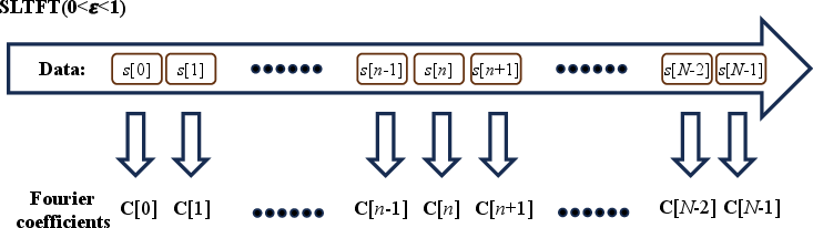
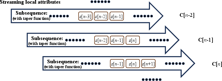
This could lead to a small time-shift in the time-frequency domain. To avoid the time-shift effect, we obtain the center-localized spectrum by implementing the streaming computation forward and backward along the time direction and adding the results together. Fig.1 illustrates the main processes of the proposed SLTFT and the streaming local attribute (Geng et al., 2024). The proposed method avoids repeatedly windowing the data, and can obtain the result streamingly all at once. Analogous to LTF decomposition (Liu and Fomel, 2013), the absolute value of $\vert\mathbf{C}[n]\vert$ represents the localized time-frequency distribution of $s[n]$, and equation 15 can be simply inverted to reconstruct the original data $s[n]$ from the coefficients $\mathbf{C}[n]$ (Fomel and Claerbout, 2016,2024):

$$\begin{aligned} s[n] =& \left( \frac{\lambda^2}{\mathbf{\Psi}[n... ...\mathbf{\Psi}^T[n]}\mathbf{\Psi}[n]\mathbf{C}[n-1]. \end{aligned}$$

The inversion using equation 16 is suffer from the trade-off between accuracy and efficiency (Fomel and Claerbout, 2024,2016). Another way to reconstruct the original data is to directly apply the equation 2. Additionally, we use an amplitude recovery factor $\alpha$ defined by

$$\alpha = \frac{s[n]}{\mathbf{\Psi}[n]\mathbf{C}[n]},$$ (17)

to ensure the amplitude unchanged. Then the amplitude-preserving coefficients $\hat{\mathbf{C}}[n]$ can be obtained by

$$\hat{\mathbf{C}}[n] = \alpha\mathbf{C}[n]=\frac{s[n]}{\mathbf{\Psi}[n]\mathbf{C}[n]}\mathbf{C}[n],$$ (18)

and the original signal $s[n]$ can be precisely reconstructed by

$$s[n] = \mathbf{\Psi}[n]\hat{\mathbf{C}}[n].$$ (19)

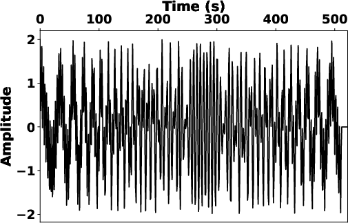
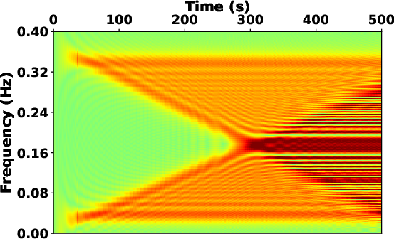
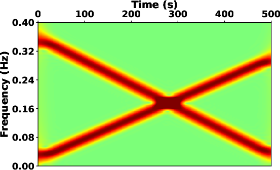
We utilize a benchmark chirp signal (see Fig.2a) to further illustrate the role of the localization scalar. Fig.2b presents the time-frequency map derived from the streaming local attribute (Geng et al., 2024), which fails in providing a localized time-frequency map if the taper function is removed to reduce the computational costs. However, the proposed SLTFT without window functions can provide a reasonable result (see Fig.2c).

Compared to the streaming local attribute with the taper function, the proposed SLTFT by updating the coefficients according to equation 15 requires only elementary algebraic operations, which effectively reduces computational cost without iteration. According to equation 9, $\mathbf{C}[n]$ is a $k\times 1$ vector and the size of $\mathbf{\Psi}[n]$ is $1\times k$ for any $n$, thus the computational complexities of $\varepsilon^2\mathbf{\Psi}[n]\mathbf{C}[n-1]\mathbf{\Psi}^T[n]$ and $s[n]\mathbf{\Psi}^T[n]$ are both $O(k)$. Meanwhile,

$$\begin{aligned} \mathbf{\Psi}[n]\mathbf{\Psi}^T[n] &= \left[\be... ...{\text{j}2\pi i (n/N)}e^{-\text{j}2\pi i (n/N)}}=k, \end{aligned}$$

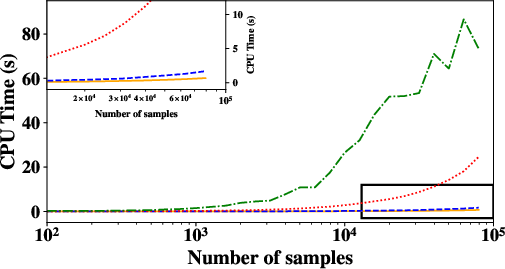
which is a constant for every $n$ and is computed only once. According to equations 15 and 18, the computational complexity of the proposed SLTFT method is 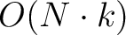$O(N\cdot k)$. Table 1 compares the complexities of different approaches, which shows the proposed method has the lowest requirement for computational resources. Fig.3 further shows the CPU time of the different methods. We select the fixed frequency sample of 500 and the fixed window length of 100 (for those who need a taper function). The number of iteration is set to 50 in the LTF decomposition. All these records are obtained by taking the average of 5 measurements. Fig.3 is visually in line with the theoretical complexity shown in table 1. It is clear that the proposed method offers a fast transform almost equivalent to the STFT and is much more efficient than the LTF decomposition and the streaming local attributes method. Moreover, it combines the advantages of flexible frequency sampling and the adaptability of time and frequency localization, which are not achievable with the STFT. This enables fast local time-frequency analysis and processing, especially for large-scale seismic data, e.g., passive seismic data (Geng et al., 2024).

streamingLTFTa,streamingLTFTb
Figure 1. Schematic illustration of (a) the proposed SLTFT and (b) the streaming local attributes method.

Table 1: Comparison of Theoretical Computational Costs among Different Methods.

cchirps,sltft,sltft1
Figure 2. Schematic illustration of (a) the synthetic chirp signal and its time-frequency map obtained by (b) the streaming local attributes without window and (c) the proposed SLTFT.

time
Figure 3. The CPU time comparison among the time-frequency analysis methods. Orange line: STFT; blue dash line: SLTFT; red dot line: streaming attributes; green dash-dot line: LTF decomposition. The convergence speed affects the CPU time of the LTF decomposition, resulting in a non-smooth curve.