plane-wave flattening

Considering that the local plane wave can be described as the following differential equation:

$$\frac{\partial u}{\partial x}+\sigma\frac{\partial u}{\partial t} = 0,$$ (3)

where $\sigma$ is the local slope in continuous space, and $u$ denotes the wavefield. In the case of the constant local slope, equation 3 has the following solution:

$$P(t,x) = f(t-\sigma),$$ (4)

where $f$ is the waveform function. In order to flatten a seismic section, we need to first select a reference trace, and then we flatten the whole profile by predicting each trace from the reference trace, following the local slope. Predicting trace $k$ from trace $r$ (reference trace) is simply:

$$\mathbf{P}_{r,k} = \mathbf{P}_{r,r+1}\cdots\mathbf{P}_{k-2,k-1}\mathbf{P}_{k-1,k}.$$ (5)

The above recursive operator $\mathbf{P}_{r,k}$ is called predictive paining (Fomel, 2010). Each $\mathbf{P}_{i,j}$ denotes the prediction operator following the local slope $\sigma$.

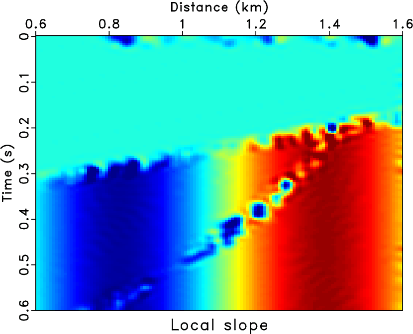
The local slope can be obtained by solving the following equation:

$$\mathbf{D}(\sigma)\mathbf{S} = \mathbf{0},$$ (6)

where $\mathbf{S}$ is the seismic section, $\mathbf{S}=[\mathbf{s}_1\quad\mathbf{s}_2\cdots\mathbf{s}_N]^T$, $\mathbf{s}_i$ denotes $i$th trace, $[\cdot]^T$ denotes the transpose of the input matrix, and $\mathbf{D}$ is called plane-wave destruction (PWD) operator (Fomel, 2002), which has the following form:

$$\mathbf{D}(\sigma) = \left[\begin{array}{ccccc} \mathbf{I} & 0 & ... ...\ 0 & 0 & \cdots & - \mathbf{P}_{N-1,N} & \mathbf{I} \\ \end{array}\right]\;.$$ (7)

Equation 6 can be solved by iterative inversion using shaping regularization with a local smoothness constraint (Fomel, 2007). Gan et al. (2015a) used a similar methodology to provide a flattened domain for attenuating random noise using truncated singular value decomposition.

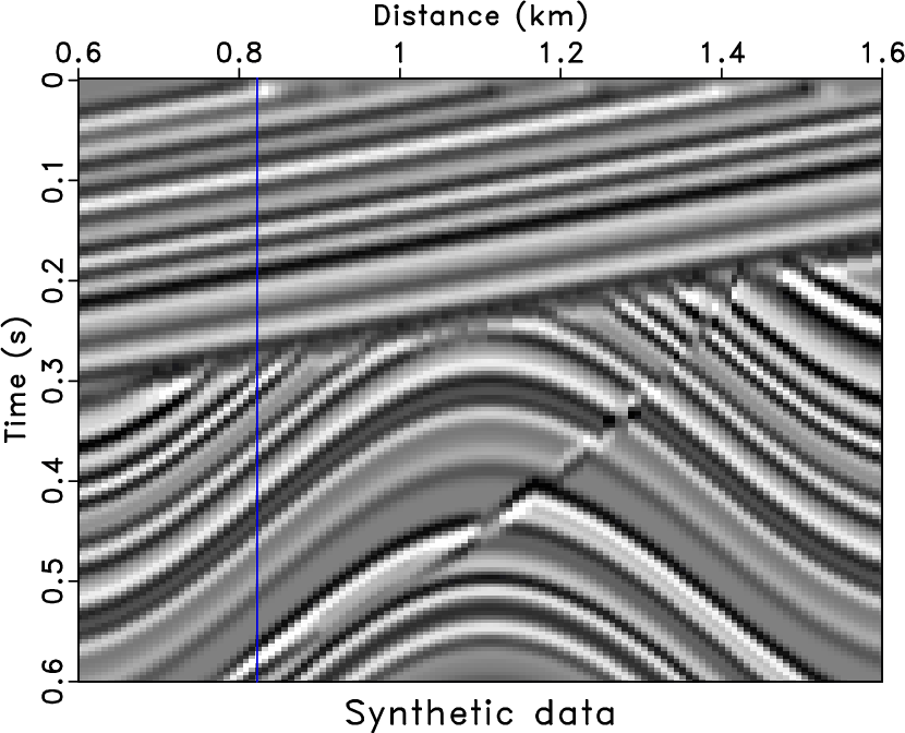
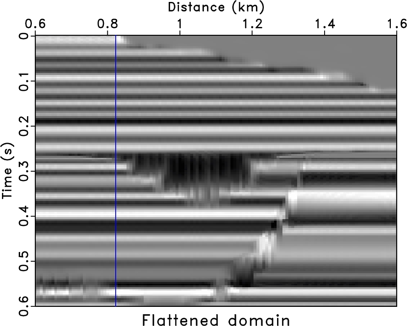
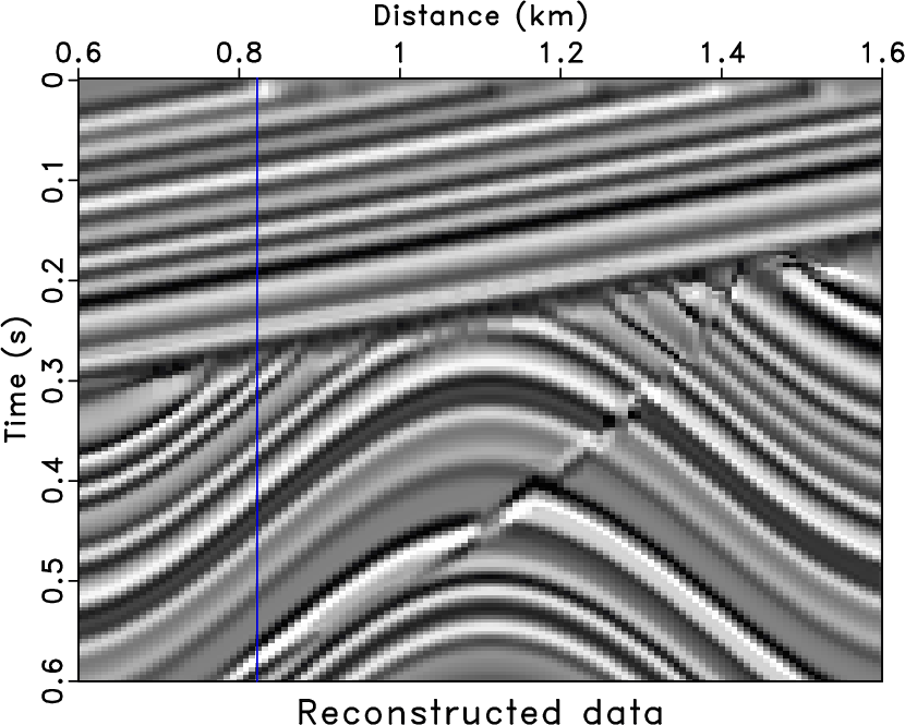
Figure 1 shows a simple demonstration of the plane-wave flattening process. Figure 1a shows a synthetic data, with dipping reflector, curved events, and faults in the profile. Figure 1b shows the corresponding local slope estimation using the PWD algorithm. Figure 1c shows the flattened domain of the synthetic data using the plane-wave flattening algorithm. The reference trace is selected as the 30th trace in the section, as highlighted by the blue line in Figures 1a, 1c and 1d. Figure 1d shows the reconstructed synthetic data using the inverse plane-wave flattening process.

sigmoid,sdip,sflat,flat-rec
Figure 1. Demonstration of the plane-wave flattening algorithm.(a) Synthetic example. (b) Local slope estimation. (c) Flattened domain. (d) Reconstructed data.