|
|
|
|
Enhancing seismic reflections using empirical mode decomposition in the flattened domain |
Next: plane-wave flattening Up: Method Previous: Method
|
|
|
|
Enhancing seismic reflections using empirical mode decomposition in the flattened domain |
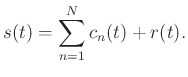
We can straightforwardly use the EMD to denoise each seismic trace because of the special frequency-decreasing property of IMF. IMFs represent different oscillations embedded in the data, and the oscillating frequency for each subsignal ![]() decreases as the sequence number of IMF gets larger. This property results from the sifting algorithm to implement the decomposition. The sifting process can be summarized as a process in which low-frequency component is gradually removed out to generate a more local-constant-frequency mode, which is followed by generating the next mode.
decreases as the sequence number of IMF gets larger. This property results from the sifting algorithm to implement the decomposition. The sifting process can be summarized as a process in which low-frequency component is gradually removed out to generate a more local-constant-frequency mode, which is followed by generating the next mode.
Chen et al. (2014b) provided an overall introduction of the applications of EMD in random noise attenuation of seismic data. According to Chen et al. (2014b), EMD can be used to denoise each 1-D signal from the 2-D seismic profile in time-space (![]() -
-![]() ) domain either along the time direction or space direction. However, because of the mode-mixing problem,
) domain either along the time direction or space direction. However, because of the mode-mixing problem, ![]() -
-![]() domain EMD along the time direction will cause some damage to useful seismic signal. A better way utilize EMD to remove noise is to apply EMD along the space direction and to remove the highly oscillating components. The frequency-space (
domain EMD along the time direction will cause some damage to useful seismic signal. A better way utilize EMD to remove noise is to apply EMD along the space direction and to remove the highly oscillating components. The frequency-space (![]() -
-![]() ) domain EMD can help to obtain faster implementation and even better performances.
) domain EMD can help to obtain faster implementation and even better performances.
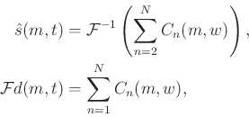
![]() EMD refers to applying EMD on
each frequency slice in the
EMD refers to applying EMD on
each frequency slice in the ![]() domain, and removing the first IMF,
which mainly represent the highest wavenumber components. The methodology can be summarized as (Chen et al., 2015a):
domain, and removing the first IMF,
which mainly represent the highest wavenumber components. The methodology can be summarized as (Chen et al., 2015a):
It is worth to be mentioned here that the ![]() EMD does not require exactly flattened events. Unlike 1D mean and median filters,
EMD does not require exactly flattened events. Unlike 1D mean and median filters, ![]() EMD can also preserve useful reflections with small dip angle. Compared with Karhunen-loeve (KL) or singular value decomposition (SVD) filtering, the
EMD can also preserve useful reflections with small dip angle. Compared with Karhunen-loeve (KL) or singular value decomposition (SVD) filtering, the ![]() EMD can be much more adaptive, because the horizontal events mainly lay in the first 1-3 IMFs after EMD in the
EMD can be much more adaptive, because the horizontal events mainly lay in the first 1-3 IMFs after EMD in the ![]() domain, however, the number of singular values corresponding to the useful horizontal reflections for KL or SVD transforms have a large range and thus is not convenient to chose. The performance for preserving horizontal events of
domain, however, the number of singular values corresponding to the useful horizontal reflections for KL or SVD transforms have a large range and thus is not convenient to chose. The performance for preserving horizontal events of ![]() EMD is also much better than that of KL or SVD transforms (Chen et al., 2015a).
EMD is also much better than that of KL or SVD transforms (Chen et al., 2015a).
|
|
|
|
Enhancing seismic reflections using empirical mode decomposition in the flattened domain |