GEO 365N/384S Seismic Data Processing Computational Assignment 5

Hyperbolic Radon transform

The parabolic Radon transform is a powerful tool but not perfectly suitable for separating hyperbolic events. An alternative tool is the time-domain hyperbolic Radon transform (also known as the velocity stack or the velocity transform). The idea of making the hyperbolic Radon transform invertible by iterative least-squares inversion was proposed by Thorson and Claerbout (1985).

1. Change directory to hw5/hradon.
2. Run

   scons -c
   

   to remove (clean) previously generated files.

   

   adj
   Figure 8. Applying the hyperbolic Radon transform. From left to right: selected CMP gather, its hyperbolic Radon transform, data reconstructed by the adjoint transform (filtered back projection).

   

   
   

4. We will use the same CMP gather as in the previous part. Figure 8 shows the selected gather, its hyperbolic Radon transform, and data reconstructed by the adjoint transform (filtered back projection). To display it on your screen, run

   scons adj.view
   

5. Use equation (1) to find the mapping of a straight line
   

   $$T(x) = \displaystyle t_0 + \frac{x}{v_0}$$ (4)

   
   
   in the hyperbolic Radon domain defined by
   

   $$\theta(x;\tau,p) = \displaystyle \sqrt{\tau^2 + p^2\,x^2}\;.$$ (5)

   
   

   

6. The program for implementing the hyperbolic Radon transform is hradon.c. This implementation includes the half-derivative filter but not any other corrections. To test if the adjoint operator is implemented correctly, you can run the dot-product test

   sfdottest ./hradon.exe np=101 dp=0.01 op=0 nx=60 dx=0.05 ox=0.287 \
   mod=rad.rsf dat=cmp.rsf
   

   The output should display a pair of numbers equal to six digits of accurate. You can run the test multiple times.

   

   inv
   Figure 9. Applying the hyperbolic Radon transform. From left to right: selected CMP gather, its hyperbolic Radon transform (using iterative least-squares inversion), data reconstructed by the inverse transform.

   

   
   

7. The adjoint operation does not reconstruct the data exactly. To achieve a better reconstruction, we can run iterative least-squares inversion using the method of conjugate gradients. The result is shown in Figure 9. To display it on your screen, run

   scons inv.view
   

8. (EXTRA CREDIT) The computational cost of the method is proportional to the number of conjugate-gradient iterations. For an extra credit, you can improve it by using preconditioning by diagonal weighting. Appropriate weights can be found by experimentation or by using the asymptotic theory (Fomel, 2003).

   

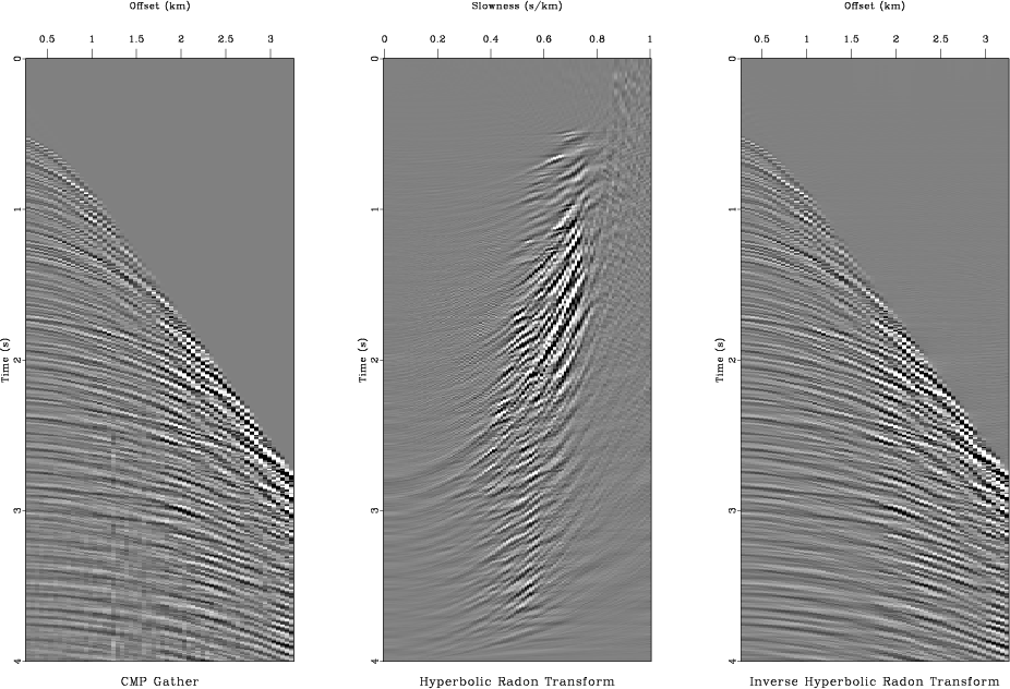
   nmorad
   Figure 10. Applying the hyperbolic Radon transform after NMO with the primary velocity trend. From left to right: selected CMP gather after NMO, hyperbolic Radon transform (using iterative least-squares inversion), data reconstructed by the inverse transform.

   

   
   

   

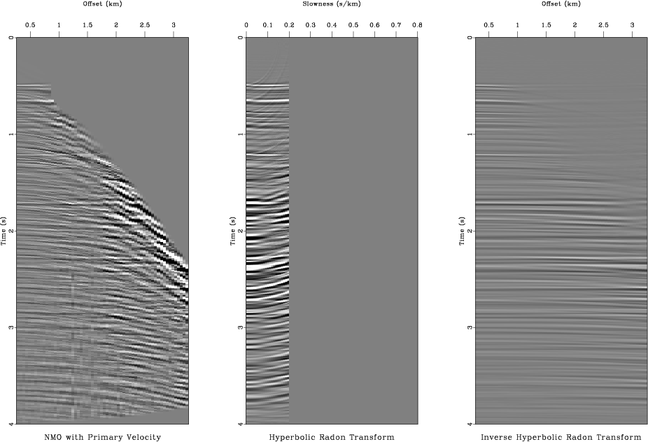
   nmocut
   Figure 11. Isolating signal in the hyperbolic Radon domain. From left to right: hyperbolic Radon transform, isolated nearly-flat events, signal reconstructed by the inverse transform.

   

   
   

   

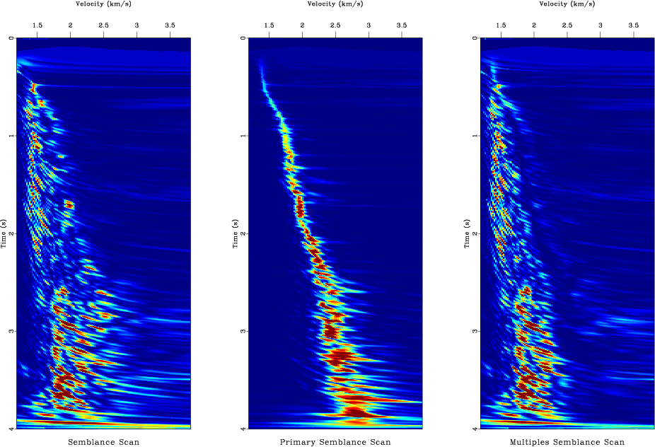
   inmo,pvscan
   Figure 12. Separating signal (primary reflections) and noise (multiple reflections). (a) From left to right: input CMP gather, estimated primaries, estimated multiples. (b) Velocity analysis using semblance scan. From left to right: using all data, using estimated primaries, using estimated multiples.

   

   
   

9. To separate primaries from multiples, we can adopt the strategy similar to the one used with the parabolic Radon:
   1. Pick the primary velocity trend.
   2. Apply NMO.
   3. Isolate nearly-flat events in the transformed domain.
   4. Transform back.
   5. Apply inverse NMO.

   The hyperbolic Radon transform is shown in Figure 10 and the output of the procedure described above is shown in Figure 12. To reproduce them on your screen, run

   scons inmo.view pvscan.view
   

10. Name some theoretical advantages and disadvantages of using the hyperbolic Radon transform in comparison with the parabolic Radon transform.

11. As before, your creative task is to try improving the results by changing the parameters in the current strategy or by changing the strategy.

/* Hyperbolic Radon transform */
#include <rsf.h>

int main(int argc, char* argv[])
{
    sf_map4 map;
    int it,nt, ix,nx, ip,np, i3,n3;
    bool adj;
    float t0,dt,t, x0,dx,x, p0,dp,p;
    float **cmp, **rad, *trace;
    sf_file in, out;

    sf_init(argc,argv);
    in = sf_input("in");
    out = sf_output("out");

    if (!sf_histint(in,"n1",&nt)) sf_error("No n1=");
    if (!sf_histfloat(in,"o1",&t0)) sf_error("No o1=");
    if (!sf_histfloat(in,"d1",&dt)) sf_error("No d1=");

    n3 = sf_leftsize(in,2);

    if (!sf_getbool("adj",&adj)) adj=false;
    /* adjoint flag */

    if (adj) {
	if (!sf_histint(in,"n2",&nx))   sf_error("No n2=");
	if (!sf_histfloat(in,"o2",&x0)) sf_error("No o2=");
	if (!sf_histfloat(in,"d2",&dx)) sf_error("No d2=");

	if (!sf_getint("np",&np)) sf_error("Need np=");
	if (!sf_getfloat("op",&p0)) sf_error("need p0=");
	if (!sf_getfloat("dp",&dp)) sf_error("need dp=");

	sf_putint(out,"n2",np);
	sf_putfloat(out,"o2",p0);
	sf_putfloat(out,"d2",dp);	
    } else {
	if (!sf_histint(in,"n2",&np))   sf_error("No n2=");
	if (!sf_histfloat(in,"o2",&p0)) sf_error("No o2=");
	if (!sf_histfloat(in,"d2",&dp)) sf_error("No d2=");

	if (!sf_getint("nx",&nx)) sf_error("Need nx=");
	if (!sf_getfloat("ox",&x0)) sf_error("need x0=");
	if (!sf_getfloat("dx",&dx)) sf_error("need dx=");

	sf_putint(out,"n2",nx);
	sf_putfloat(out,"o2",x0);
	sf_putfloat(out,"d2",dx);
    }

    trace = sf_floatalloc(nt);
    cmp = sf_floatalloc2(nt,nx);
    rad = sf_floatalloc2(nt,np);

    /* initialize half-order differentiation */
    sf_halfint_init (true,nt,1.0f-1.0f/nt);

    /* initialize spline interpolation */
    map = sf_stretch4_init (nt, t0, dt, nt, 0.01);
    
    for (i3=0; i3 < n3; i3++) { 
	if( adj) {
	    for (ix=0; ix < nx; ix++) { 
		sf_floatread(trace,nt,in);
		sf_halfint_lop(true,false,nt,nt,cmp[ix],trace);
	    }
	} else {	    
	    sf_floatread(rad[0],nt*np,in);	    
	}

	sf_adjnull(adj,false,nt*np,nt*nx,rad[0],cmp[0]);
	
	for (ip=0; ip < np; ip++) { 
	    p = p0 + ip*dp;
	    for (ix=0; ix < nx; ix++) { 
		x = x0 + ix*dx;
		
		for (it=0; it < nt; it++) {		
		    t = t0 + it*dt;
		    trace[it] = hypotf(t,p*x);
                    /* hypot(a,b)=sqrt(a*a+b*b) */
		}

		sf_stretch4_define(map,trace);
		
		if (adj) {
		    sf_stretch4_apply_adj(true,map,rad[ip],cmp[ix]);
		} else {
		    sf_stretch4_apply    (true,map,rad[ip],cmp[ix]);
		}
	    }
	}

	if( adj) {
	    sf_floatwrite(rad[0],nt*np,out);
	} else {
	    for (ix=0; ix < nx; ix++) {
		sf_halfint_lop(false,false,nt,nt,cmp[ix],trace);
		sf_floatwrite(trace,nt,out);
	    }
	}
    }

    exit(0);
}

from rsf.proj import *

# Download one CMP gather (with mute)
Fetch('cmp.HH','viking')

Flow('cmp','cmp.HH','dd form=native')
Plot('cmp','grey title="CMP Gather" clip=8.66')

prog = Program('hradon.c')
hradon = str(prog[0])

Flow('rad',['cmp',hradon],
     './${SOURCES[1]} adj=y np=101 dp=0.01 op=0')
Plot('rad',
     '''
     grey title="Hyperbolic Radon Transform" 
     label2=Slowness unit2=s/km
     ''')

Flow('adj',['rad',hradon],
     './${SOURCES[1]} adj=n nx=60 dx=0.05 ox=0.287')
Plot('adj','grey title="Adjoint Hyperbolic Radon Transform" ')

Result('adj','cmp rad adj','SideBySideAniso')

Flow('inv',['cmp',hradon,'rad'],
     '''
     conjgrad ./${SOURCES[1]} mod=${SOURCES[2]} 
     np=101 dp=0.01 op=0 nx=60 dx=0.05 ox=0.287 niter=10
     ''')
Plot('inv',
     '''
     grey title="Hyperbolic Radon Transform" 
     label2=Slowness unit2=s/km
     ''')

Flow('cmp2',['inv',hradon],
     './${SOURCES[1]} adj=n nx=60 dx=0.05 ox=0.287')
Plot('cmp2',
     'grey title="Inverse Hyperbolic Radon Transform" clip=8.66')

Result('inv','cmp inv cmp2','SideBySideAniso')

# Velocity scan

Flow('vscan','cmp',
     'vscan semblance=y half=n v0=1.2 nv=131 dv=0.02')
Plot('vscan',
     'grey color=j allpos=y title="Semblance Scan" unit2=km/s')

# Automatic pick

Flow('vpick','vscan',
     '''
     mutter inner=y x0=1.4 half=n v0=0.45 t0=0.5 | 
     pick rect1=50 vel0=1.5
     ''')
Plot('vpick',
     '''
     graph yreverse=y transp=y plotcol=7 plotfat=7 
     pad=n min2=1.2 max2=3.8 wantaxis=n wanttitle=n
     ''')

Plot('vscan2','vscan vpick','Overlay')

# NMO

Flow('nmo','cmp vpick','nmo half=n velocity=${SOURCES[1]}')
Plot('nmo','grey title="NMO with Primary Velocity" clip=9.83')

Result('vscan','cmp vscan2 nmo','SideBySideAniso')

Flow('nmorad0',['cmp',hradon],
     './${SOURCES[1]} adj=y np=161 dp=0.005 op=0')
Flow('nmorad',['nmo',hradon,'nmorad0'],
     '''
     conjgrad ./${SOURCES[1]} mod=${SOURCES[2]} 
     np=161 dp=0.005 op=0 nx=60 dx=0.05 ox=0.287 niter=10
     ''')
Plot('nmorad',
     '''
     grey title="Hyperbolic Radon Transform" 
     label2=Slowness unit2=s/km
     ''')

Flow('nmo2',['nmorad',hradon],
     './${SOURCES[1]} adj=n nx=60 dx=0.05 ox=0.287')
Plot('nmo2',
     'grey title="Inverse Hyperbolic Radon Transform" clip=9.83')

Result('nmorad','nmo nmorad nmo2','SideBySideAniso')

Flow('cut','nmorad','cut min2=0.2')
Plot('cut',
     '''
     grey title="Hyperbolic Radon Transform" 
     label2=Slowness unit2=s/km
     ''')

Flow('signal',['cut',hradon],
     './${SOURCES[1]} adj=n nx=60 dx=0.05 ox=0.287')
Plot('signal',
     'grey title="Inverse Hyperbolic Radon Transform" clip=9.83')

Result('nmocut','nmo cut signal','SideBySideAniso')

# Inverse NMO

Flow('inmo','signal vpick',
     'inmo half=n velocity=${SOURCES[1]} | mutter half=n v0=1.2')
Plot('inmo','grey title=Signal clip=8.66')

Flow('pvscan','inmo',
     'vscan semblance=y half=n v0=1.2 nv=131 dv=0.02')
Plot('pvscan',
     'grey color=j allpos=y title="Primary Semblance Scan" ')

Flow('mult','cmp inmo','add scale=1,-1 ${SOURCES[1]}')
Plot('mult','grey title=Noise clip=8.66')

Flow('mvscan','mult',
     'vscan semblance=y half=n v0=1.2 nv=131 dv=0.02')
Plot('mvscan',
     'grey color=j allpos=y title="Multiples Semblance Scan" ')

Result('inmo','cmp inmo mult','SideBySideAniso')
Result('pvscan','vscan pvscan mvscan','SideBySideAniso')

End()

GEO 365N/384S Seismic Data Processing Computational Assignment 5