Random noise attenuation using $f$-$x$ regularized nonstationary autoregression

Field poststack dataset

data,fxm,tx,npre
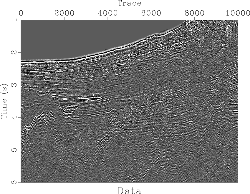
Figure 6. (a) A field marine data set. (b) The result of $f$-$x$ domain prediction. (c) The result of $t$-$x$ domain prediction. (d) The result of $f$-$x$ RNA.

fxdiff,txdiff,nprediff
Figure 7. Difference sections of $f$-$x$ domain prediction (a), $t$-$x$ domain prediction (b), and $f$-$x$ RNA (c).

zdata,zfxm,ztx,znpre
Figure 8. Zoomed sections. (a) Original data. (b) The result of $f$-$x$ domain prediction. (c) The result of $t$-$x$ domain prediction. (d) The result of $f$-$x$ RNA.

dataf,fxf,txf,npref
Figure 9. Comparison on spectra of one trace at 6000 m in field marine data (Figure 6(a)- 6(d)). (a)-(d) are the amplitude spectra of one trace at 6000 m in Figures 6(a)- 6(d), respectively.

Figure 6(a) is a seismic image from marine data after time migration. The preprocessing, such as bandpass filtering and migration, has removed some noise. However, some noise still exists in this image (indicated by arrows). This dataset is not structurally too complex and the noise seems random. Therefore, we can use $t$-$x$ domain or $f$-$x$ domain prediction methods to attenuate the random noise. Figures 6(b)- 6(d) show the results of random noise attenuation using $f$-$x$ domain prediction, $t$-$x$ domain prediction and $f$-$x$ RNA, respectively. The length of time window is 512 ms in all the three methods. For $f$-$x$ RNA, the filter length is $M=4$, and the smoothing radiuses in space and frequency axes are respectively 20 and 3, ${{r}_{x}}=20$, ${{r}_{f}}=3$. The $f$-$x$ domain prediction is implemented over a sliding window of 20 traces width with 50% overlap and the filter length is $M=4$ and the $t$-$x$ domain prediction is implemented over the same sliding window and the filter length in space and time are 6 and 5 respectively. The $f$-$x$ domain and $t$-$x$ domain prediction methods removes random noise well in the case that the events are approximately linear. In the area of complex structure, however, both of the $f$-$x$ domain and $t$-$x$ domain prediction methods can not obtain a good result. Compared to $f$-$x$ domain and $t$-$x$ domain prediction methods, $f$-$x$ RNA removes more noise and preserves signals (Figure 7(a)- 7(c)). Note that $f$-$x$ domain and $t$-$x$ domain prediction methods remove some signals, especially for complex structure (indicated by arrows in Figures 7(a) and 7(b)). We display the zoomed section in Figure 8(a)- 8(d). The zoomed sections show the proposed method is more effective than other methods, especially in the area of complex structure indicated by arrow. The $f$-$x$ RNA gives a good result not only for linear events but also for curving events (indicated by arrows in Figure 8(a)- 8(d)). From the comparison on the spectra of a trace randomly chosen as shown in Figure 9(a)- 9(d), we can see that $f$-$x$ domain and $t$-$x$ domain prediction methods greatly attenuate frequency components in [10,30] Hz, which includes effective signals. Thus, the difference sections of $f$-$x$ domain and $t$-$x$ domain prediction methods (Figures 7(a) and 7(b)) include more signals than $f$-$x$ RNA (Figure 7(c)). For high frequency random noise, all the three methods can achieve a similar result (Figure 9(a)- 9(d)).

Random noise attenuation using $f$-$x$ regularized nonstationary autoregression