Guide to RSF file format

This page was created from the LaTeX source in book/rsf/rsf/format.tex using latex2wiki

Principles

The main design principle behind the RSF data format is KISS ("Keep It Short and Simple"). The RSF format is borrowed from the SEPlib data format originally designed at the Stanford Exploration Project (Claerbout, 1991). The format is made as simple as possible for maximum convenience, transparency and flexibility. According to the Unix tradition, common file formats should be in a readable textual form so that they can be easily examined and processed with universal tools. Raymond (2004) writes:

To design a perfect anti-Unix, make all file formats binary and opaque, and require heavyweight tools to read and edit them.

If you feel an urge to design a complex binary file format, or a complex binary application protocol, it is generally wise to lie down until the feeling passes.

Storing large-scale datasets in a text format may not be economical. RSF chooses the next best thing: it allows data values to be stored in a binary format but puts all data attributes in text files that can be read by humans and processed with universal text-processing utilities.

Example

Let us first create some synthetic RSF data.

bash$ sfmath n1=1000 output='sin(0.5*x1)' > sin.rsf

Open and read the file sin.rsf.

bash$ cat sin.rsf
sfmath  rsf/rsf/rsftour:        fomels@egl      Sun Jul 31 07:18:48 2005

        o1=0
        data_format="native_float"
        esize=4
        in="/tmp/sin.rsf@"
        x1=0
        d1=1
        n1=1000

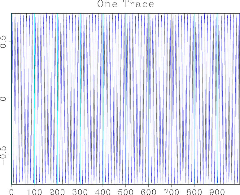
The file contains nine lines with simple readable text. The first line shows the name of the program, the working directory, the user and computer that created the file and the time it was created (that information is recorded for accounting purposes). Other lines contain parameter-value pairs separated by the "=" sign. The "in" parameter points to the location of the binary data. Before we discuss the meaning of parameters in more detail, let us plot the data.

bash$ < sin.rsf  sfwiggle title='One Trace' | sfpen

On your screen, you should see a plot similar to the figure below.

An example sinusoid plot.

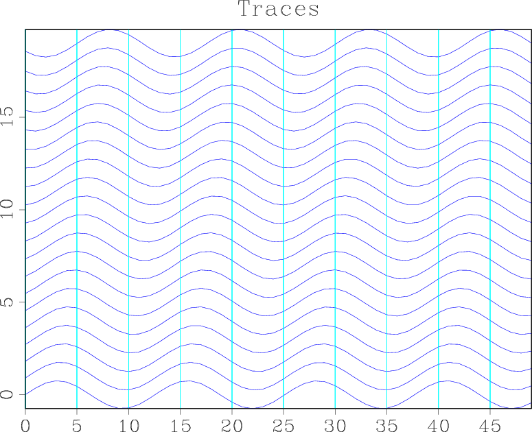
Suppose you want to reformat the data so that instead of one trace of a thousand samples, it contains twenty traces with fifty samples each. Try running

bash$ < sin.rsf sed 's/n1=1000/n1=50 n2=20/' > sin10.rsf 
bash$ < sin10.rsf sfwiggle title=Traces | sfpen

or (using pipes)

bash$ < sin.rsf sed 's/n1=1000/n1=50 n2=20/' | sfwiggle title=Traces | sfpen

On your screen, you should see a plot similar to the figure below:

An example sinusoid plot, with data reformatted to twenty traces.

What happened? We used sed, a standard Unix line editing utility to change the parameters describing the data dimensions. Because of the simplicity of this operation, there is no need to create specialized data formatting tools or to make the sfwiggle program accept additional formatting parameters. Other general-purpose Unix tools that can be applied on RSF files include cat, echo, grep, etc. An alternative way to obtain the previous result is to run

bash$ ( cat sin.rsf; echo n1=50 n2=20 ) > sin10.rsf 
bash$ < sin10.rsf sfwiggle title=Traces | sfpen

In this case, the cat utility simply copies the contents of the previous file, and the echo utility appends new line "n1=50 n2=20". A new value of the n1 parameter overwrites the old value of n1=1000, and we achieve the same result as before. Of course, one could also edit the file by hand with one of the general purpose text editors. For recording the history of data processing, it is usually preferable to be able to process files with non-interactive tools.

Header and Data files

A simple way to check the layout of an RSF file is with the sfin program.

bash$ sfin sin10.rsf
sin10.rsf:
    in="/tmp/sin.rsf@"
    esize=4 type=float form=native
    n1=50          d1=1           o1=0
    n2=20          d2=?           o2=?
        1000 elements 4000 bytes

The program reports the following information: the location of the data file (/tmp/sin.rsf\@), the element size (4 bytes), the element type (floating point), the element form (native), the hypercube dimensions ($50\times 20$), axis scaling (1 and unspecified), and axis origin (0 and unspecified). It also checks the total number of elements and bytes in the data file. Let us examine this information in detail. First, we can verify that the data file exists and contains the specified number of bytes:

bash$ ls -l /tmp/sin.rsf@
-rw-r--r--  1 sergey users 4000 2004-10-04 00:35 /tmp/sin.rsf@

4000 bytes in this file are required to store $50\times 20$ floating-point 4-byte numbers in a binary form. Thus, the data file contains nothing but the raw data in a contiguous binary form.

Datapath

How did the RSF program (sfmath) decide where to put the data file? In the order of priority, the rules for selecting the data file name and the data file directory are as follows:

1. Check --out= parameter on the command line. The parameter specifies the output data file location explicitly.
2. Specify the path and the file name separately.
   • The rules for the path selection are:
     1. Check datapath= parameter on the command line. The parameter specifies a string to prepend to the file name. The string may contain the file directory.
     2. Check DATAPATH environmental variable. It has the same meaning as the parameter specified with datapath=.
     3. Check for .datapath file in the current directory. The file may contain a line

         datapath=/path/to_file/ 

        or

         machine_name datapath=/path/to_file/ 

        if you indent to use different paths on different platforms.
     4. Check for .datapath file in the user home directory.
     5. Put the data file in the current directory (similar to datapath=./).

   • The rules for the filename selection are:
     1. If the output RSF file is in the current directory, the name of the data file is made by appending \@.
     2. If the output file is not in the current directory or if it is created temporarily by a program, the name is made by appending random characters to the name of the program and selected to be unique.

Examples:

bash$ sfspike n1=10 out=test1 > spike.rsf 
bash$ grep in spike.rsf         
in="test1" 

bash$ sfspike n1=10 datapath=/tmp/ > spike.rsf 
bash$ grep in spike.rsf         
in="/tmp/spike.rsf@" 

bash$ DATAPATH=/tmp/ sfspike n1=10 > spike.rsf 
bash$ grep in spike.rsf         
in="/tmp/spike.rsf@" 

bash$ sfspike n1=10 datapath=/tmp/ > /tmp/spike.rsf 
bash$ grep in /tmp/spike.rsf 
in="/tmp/sfspikejcARVf" 

Packing header and data together

While the header and data files are separated by default, it is also possible to pack them together into one file. To do that, specify the program's "--out" parameter as --out=stdout. Example:

bash$ sfspike n1=10 --out=stdout > spike.rsf
bash$ grep in spike.rsf
Binary file spike.rsf matches
bash$ sfin spike.rsf
spike.rsf:
    in="stdin"
    esize=4 type=float form=native
    n1=10          d1=0.004       o1=0          label1="Time" unit1="s"
        10 elements 40 bytes
bash$ ls -l spike.rsf
-rw-r--r--  1 sergey users 196 2004-11-10 21:39 spike.rsf

If you examine the contents of spike.rsf, you will find that it starts with the text header information, followed by special symbols, followed by binary data. Packing headers and data together may not be a good idea for data processing but it works well for storing data: it is easier to move the packed file around than to move two different files (header and binary) together while remembering to preserve their connection. Packing header and data together is also the current mechanism used to push RSF files through Unix pipes.

Type

The data stored with RSF can have different types: character, unsigned character, integer, floating point, or complex. By default, single precision is used for numbers (int and float data types in the C programming language). The number of bytes required for represent these numbers may depend on the platform.

Form

The data stored with RSF can also be in a different form: ASCII, native binary, and XDR binary. Native binary is often used by default. It is the binary format employed by the machine that is running the application. On Linux-running PC, the native binary format will typically correspond to the so-called little-endian byte ordering. On some other platform, it might be big-endian ordering. XDR is a binary format designed by Sun for exchanging files over network. It typically corresponds to big-endian byte ordering. It is more efficient to process RSF files in the native binary format but, if you intend to access data from different platforms, it might be a good idea to store the corresponding file in an XDR format. RSF also allows for an ASCII (plain text) form of data files. Conversion between different types and forms is accomplished with sfdd program. Here are some examples. First, let us create synthetic data.

bash$ sfmath n1=10 output='10*sin(0.5*x1)' > sin.rsf
bash$ sfin sin.rsf
sin.rsf:
    in="/tmp/sin.rsf@"
    esize=4 type=float form=native
    n1=10          d1=1           o1=0
        10 elements 40 bytes
bash$ < sin.rsf sfdisfil
   0:             0        4.794        8.415        9.975        9.093
   5:         5.985        1.411       -3.508       -7.568       -9.775

Converting the data to the integer type:

bash$ < sin.rsf sfdd type=int > isin.rsf
bash$ sfin isin.rsf
isin.rsf:
    in="/tmp/isin.rsf@"
    esize=4 type=int form=native
    n1=10          d1=1           o1=0
        10 elements 40 bytes
bash$ < isin.rsf sfdisfil
   0:    0    4    8    9    9    5    1   -3   -7   -9

Converting the data to the ASCII form:

bash$ < sin.rsf sfdd form=ascii > asin.rsf
bash$ < asin.rsf sfdisfil
   0:             0        4.794        8.415        9.975        9.093
   5:         5.985        1.411       -3.508       -7.568       -9.775
bash$ sfin asin.rsf
asin.rsf:
    in="/tmp/asin.rsf@"
    esize=0 type=float form=ascii
    n1=10          d1=1           o1=0
        10 elements
bash$ cat /tmp/asin.rsf@
0 4.79426 8.41471 9.97495 9.09297 5.98472 1.4112 -3.50783
-7.56803 -9.7753

Hypercube

While RSF stores binary data in a contiguous 1-D array, the conceptual data model is a multidimensional hypercube. By convention, the dimensions of the cube are defined with parameters n1, n2, n3, etc. The fastest axis is n1. Additionally, the grid sampling can be given by parameters d1, d2, d3, etc. The axes origins are given by parameters o1, o2, o3, etc. Optionally, you can also supply the axis label strings label1, label2, label3, etc., and axis units strings unit1, unit2, unit3, etc.

Compatibility with other file formats

It is possible to exchange RSF-formatted data with other popular data formats.

Compatibility with SEPlib

RSF is mostly compatible with its predecessor, the SEPlib file format. However, there are several important differences:

1. SEPlib programs typically use the element size (esize= parameter) to distinguish between different data types: esize=4 corresponds to floating point data, while esize=8 corresponds to complex data. The RSF type handling mechanism is different: data types are determined from the value of the data_format parameter. Madagascar computational programs typically output files with data_format="native_float" or native_complex.
2. The default data form in SEPlib programs is typically XDR and not native as it is in RSF. Thus, to make a dataset created with SEPlib readable by Madagascar programs, you would typically need to add to the history file data_format="xdr_float" or data_format="xdr_complex" .
3. It is possible to pipe the output of Madagascar programs to SEPlib:

   bash$ sfspike n1=1 | Attr want=min

   (output should be: minimum value = 1 at 1). However, piping the output of SEPlib programs to RSF (or, for that matter, any other non-SEPlib programs) will result in an unterminated process. For example, the command

    bash$ Spike n1=1 | sfattr want=min 

   will hang. This is because SEPlib uses sockets for piping and expects a socket connection from the receiving program, while Madagascar passes data through regular Unix pipes.
4. SEP3D is an extension of SEPlib for operating with irregularly sampled data (Biondi et al., 1996). There is no equivalent of it in RSF for the reasons explained in the beginning of this guide. Operations with irregular datasets are supported through the use of auxiliary input files that represent the geometry information.

Notes

Reading and writing SEG-Y and SU files

The SEG-Y format is based on the proposal of Barry et al. (1975). It was revised in 2002. The SU format is a modification of SEG-Y used in Seismic Unix (Stockwell, 1997). To convert files from SEG-Y or SU format to RSF, use the sfsegyread program. Let us first manufacture an example file using SU utilities (Stockwell, 1999):

bash$ suplane > plane.su
bash$ segyhdrs < plane.su | segywrite tape=plane.segy

To convert it to RSF, use either

bash$ sfsuread < plane.su tfile=tfile.rsf endian=0 > plane.rsf

or

bash$ sfsegyread < plane.segy tfile=tfile.rsf \
hfile=hfile bfile=bfile > plane.rsf

The endian flag is needed if the SU file originated from a little-endian machine such as Linux PC. Several files are generated. The standard output contains an RSF file with the data (32 traces with 64 samples each):

bash$ sfin plane.rsf
plane.rsf:
    in="/tmp/plane.rsf@"
    esize=4 type=float form=native
    n1=64          d1=0.004       o1=0
    n2=32          d2=?           o2=?
        2048 elements 8192 bytes

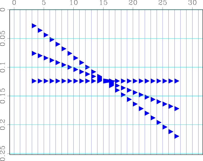
The contents of this file are displayed in the figure.

The output of suplane, converted to RSF and displayed with sfwiggle.

The tfile is an RSF integer-type file with the trace headers (32 headers with 71 traces each):

bash$ sfin tfile.rsf
tfile.rsf:
    in="/tmp/tfile.rsf@"
    esize=4 type=int form=native
    n1=71          d1=?           o1=?
    n2=32          d2=?           o2=?
        2272 elements 9088 bytes

The contents of trace headers can be quickly examined with the sfheaderattr program. The hfile is the ASCII header file for the whole record.

bash$ head -c 242 hfile
C      This tape was made at the
C                                                                              
C      Center for Wave Phenomena                         

The bfile is the binary header file.

To convert files back from RSF to SEG-Y or SU, use the sfsegywrite program and reverse the input and output:

bash$ sfsuwrite > plane.su su=y tfile=tfile.rsf endian=0 < plane.rsf

or

bash$ sfsegywrite > plane.segy tfile=tfile.rsf \
hfile=hfile bfile=bfile < plane.rsf

If hfile= and bfile= are not supplied to sfsegywrite, the corresponding headers will be generated on the fly. The trace header file can be generated with sfsegyheader. Here is an example:

bash$ sfheadermath < plane.rsf output=N+1 | sfdd type=int > tracl.rsf
bash$ sfsegyheader < plane.rsf tracl=tracl.rsf > tfile.rsf
bash$ sfsegywrite  < plane.rsf tfile=tfile.rsf > plane.segy

Reading and writing ASCII files

Reading and writing ASCII files can be accomplished with the sfdd program. For example, let us take an ASCII file with numbers

bash$ cat file.asc
1.0 1.5 3.0
4.8 9.1 7.3

Converting it to RSF is as simple as

bash$ echo in=file.asc n1=3 n2=2 data_format=ascii_float > file.rsf
bash$ sfin file.rsf
file.rsf:
    in="file.asc"
    esize=0 type=float form=ascii
    n1=3           d1=?           o1=?
    n2=2           d2=?           o2=?
        6 elements

For more efficient input/output operations, it might be advantageous to convert the data type to native binary, as follows:

bash$ echo in=file.asc n1=3 n2=2 data_format=ascii_float | \
sfdd form=native > file.rsf
bash$ sfin file.rsf
file.rsf:
    in="/tmp/file.rsf@"
    esize=4 type=float form=native
    n1=3           d1=?           o1=?
    n2=2           d2=?           o2=?
        6 elements 24 bytes

Convert from RSF to ASCII is equally simple:

bash$ sfdd form=ascii out=file.asc < file.rsf > /dev/null
bash$ cat file.asc
1 1.5 3 4.8 9.1 7.3

You can use the line= and format= parameters in sfdd to control the ASCII formatting:

bash$ sfdd form=ascii out=file.asc \
line=3 format="%3.1f " < file.rsf > /dev/null
bash$ cat file.asc
1.0 1.5 3.0
4.8 9.1 7.3

An alternative is to use sfdisfil.

bash$ sfdisfil > file.asc col=3 format="%3.1f " number=n < file.rsf
bash$ cat file.asc
1.0 1.5 3.0
4.8 9.1 7.3

Other documentation

This note should give you a general understanding of the RSF file format. See the RSF Comprehensive Description if you are interested in minutia. Other relevant documentation is:

• Why Madagascar
• Installation instructions
• Madagascar self-documentation
• Guide to madagascar programs
• Guide to the Madagascar programming interface
• Guide to programming with madagascar
• Revisiting SEP tour with Madagascar and SCons
• Reproducible computational experiments using SCons

About this document

This page was created from the LaTeX source in book/rsf/rsf/format.tex using latex2wiki.

References

- ↑ Claerbout, J. F., 1991, Introduction to Seplib and SEP utility software, in SEP-70, 413--436. Stanford Exploration Project.
- ↑ Raymond, E. S., 2004, The art of UNIX programming: Addison-Wesley.
- ↑ Biondi, B., R. Clapp, and S. Crawley, 1996, SEPlib90: SEPlib for 3-D prestack data, in SEP-92, 343--364. Stanford Exploration Project.
- ↑ Barry, K. M., D. A. Cavers, and C. W. Kneale, 1975, Report on recommended standards for digital tape formats: Geophysics, 40, 344--352
- ↑ See http://www.seg.org/SEGportalWEBproject/prod/SEG-Publications/Pub-Technical-Standards/Documents/seg_y_rev1.pdf
- ↑ Stockwell, J. W., 1997, Free software in education: A case study of CWP/SU: Seismic Unix: The Leading Edge, 16, 1045--1049.
- ↑ -------- 1999, The CWP/SU: Seismic Un*x package: Computers and Geosciences, 25, 415--419.