A new paper is added to the collection of reproducible documents:
Modeling of pseudo-acoustic P-waves in orthorhombic media with a lowrank approximation
Lowrank modeling in orthorhombic media
June 25, 2013 Documentation No comments
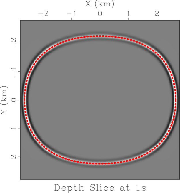
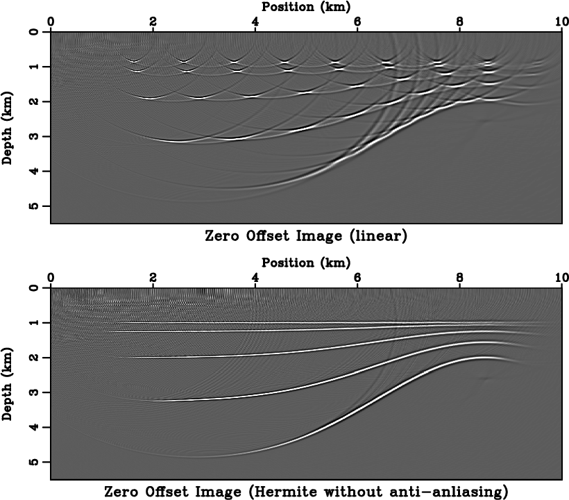
Kirchhoff migration with traveltime source-derivatives
June 24, 2013 Documentation No comments
A new paper is added to the collection of reproducible documents:
Kirchhoff migration using eikonal-based computation of traveltime source-derivatives
Extending MATLAB interface
June 13, 2013 Systems No comments
For those using MATLAB interface to Madagascar, a new function, m8r, allows running Madagascar programs and workflows directly on MATLAB objects. The following MATLAB code runs regularized time-frequency analysis using sftimefreq:
% create chirp signal
t=0:0.001:1;
y=chirp(t,100,1,25,'q',[],'convex');

% spectragram analysis in MATLAB
spectrogram(y,256,200,256,1000);
set(gca,'xlim',[0,250]);
set(gca,'ydir','reverse');
ylabel('Time (s)');

% time-frequency analysis in Madagascar
tf = m8r('sftimefreq rect=50 nw=251 dw=1',y',0.001);

f = 0:250;
imagesc(t,f,tf);
xlabel('Frequency (Hz)');
ylabel('Time (s)');

Program of the month: sfwiggle
June 12, 2013 Programs No comments
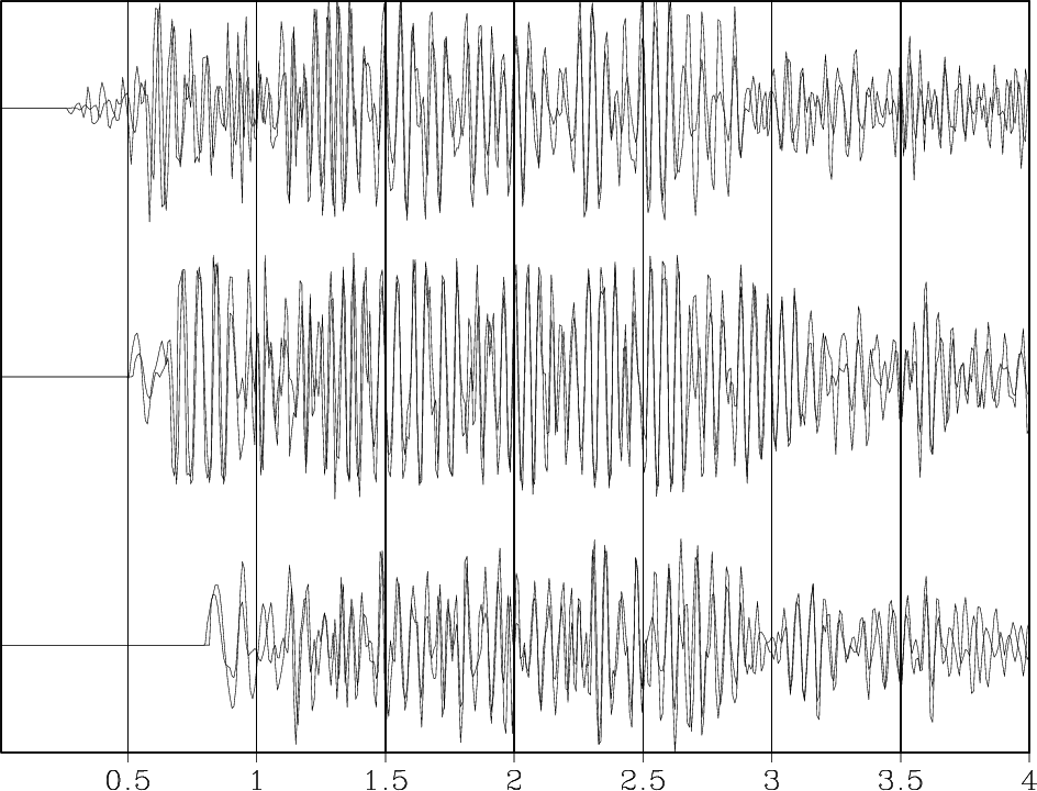
sfwiggle plots data using the traditional seismic method of wiggly traces.
The following example from rsf/rsf/rsftour shows a typical output:

Similarly to other plotting programs, there are multiple parameters that control the output. For example, poly=y draws solid polygons for highlighting positive data, transp=y transposes the two axes, xreverse=y or yreverse=y reverse the corresponding axis. Data scaling is controlled with either the absolute clip (clip=) or percentage clip (pclip=).
The following example uses transp=y poly=y yreverse=y pclip=100 unit2=km unit1=s label1=Time label2=Offset:

Use seemean=y to display lines corresponding to the mean value, use zplot= to control relative separation between different traces (the default is 0.75). The following example from bei/sg/toldi uses zplot=0.4:
Finally, sfwiggle makes it possible to plot irregularly sampled data by providing trace coordinates in xpos= file and (optionally) coordinate range with xmin= and xmax=. The following example from jsg/avo/avo2 shows a seismic gather displayed with (a) sfgrey in trace-number coordinates and (b) sfwiggle in offset coordinates.

10 previous programs of the month:
Elastic wave equations on GPU
June 11, 2013 Documentation No comments
A new paper is added to the collection of reproducible documents:
Solving 3D anisotropic elastic wave equations on parallel GPU devices
This is the first contribution from the University of Western Australia.

Program of the month: sfvscan
May 4, 2013 Programs No comments
sfvscan implements seismic velocity analysis by scanning stacking velocities. This transformation is also known as the velocity transform or the hyperbolic Radon transform.
The following example from bei/vela/vscan shows an example for transforming a CMP (common midpoint) gather to a velocity (actually slowness) scan.

By default, sfvscan uses velocity as the horizontal axis. To change it to slowness, use slowness=y. It is also possible to use velocity or slowness squared by specifying squared=y. The range of velocities or slownesses to scan is given by v0=, dv=, nv=. In addition, it is possible to scan heterogeneity parameters in the shifted-hyperbola approximation using smax= and ns=.
The offset range in the input file is specified similarly to how it is done in sfnmo: The offset can be either regular (specified as the second axis in the input file) or irregular (specified in offset= file). By default, half-offset is used. To use full offset, specify half=n. Additionally, it is possible to specify a mask (with mask= file containing 1s and 0s) for skipping certain input traces during the scan.
The NMO correction involved in velocity scanning is associated with the phenomenon of “NMO stretch”, a non-linear stretching of time at large offsets. The maximum allowed relative stretch is controlled by str= parameter. The part of the data that is stretched more than the allowed stretch gets muted. The width of the mute zone is controlled by mute= parameter.
By default, sfvscan outputs simple stack. To output semblance instead, use semblance=y or type=semblance. It is also possible to output other kinds of semblance attributes: differential semblance (type=w), AB semblance (type=a), or weighted semblance (type=w). See
Li, J., & Symes, W. W. (2007). Interval velocity estimation via NMO-based differential semblance. Geophysics, 72(6), U75-U88.
Sarkar, D., Castagna, J. P., & Lamb, W. J. (2001). AVO and velocity analysis. Geophysics, 66(4), 1284-1293.
Sarkar, D., Baumel, R. T., & Larner, K. L. (2002). Velocity analysis in the presence of amplitude variation. Geophysics, 67(5), 1664-1672.
Fomel, S. (2009). Velocity analysis using AB semblance. Geophysical Prospecting, 57(3), 311-321.
Luo, S., & Hale, D. (2012). Velocity analysis using weighted semblance. Geophysics, 77(2), U15-U22.
The following example from jsg/avo/avo2 shows a comparison between velocity scans computed using the conventional semblance and AB semblance.

For robustness, semblance values are averaged in time. The length of the averaging window in samples is given by nb= (the default is 2 time samples). By default, the input samples are stacked along the hyperbola with an asymptotically pseudounitary weight equal to the absolute value of offset times velocity. To apply a uniform weight, use weight=n. For the justification of the pseudounitary weighting, see
Claerbout, J. F., 1995, Basic Earth Imaging: Stanford Exploration Project.
S. Fomel, 2003, Asymptotic pseudounitary stacking operators: Geophysics, v. 68, 1032-1042.
For the operation inverse or adjoint to the velocity scan, use sfveltran, sfvelmod or sfvelinv.
For a faster implementation of the velocity scan (using the buttefly algorithm), use sfradon2.
From the output of the semblance scan computed with sfvscan, the velocity trend can be picked automatically with sfpick.
10 previous programs of the month
Events of the year
May 2, 2013 Celebration No comments
A Madagascar School will take place on August 15, 2013, in Melbourne, Australia, during the ASEG convention and is organized by Jeff Shragge from the University of Western Australia.

In addition, the First Madagascar Working Workshop will take place on July 25-27, 2013, in Austin, Texas. The declared objectives of the workshop are
- To expand Madagascar’s collection of reproducible papers. New reproducible papers may include papers written using Madagascar programs as well as papers written using other open-source software tools.
- To create and expand a seismic migration gallery. Migration gallery is a matrix where rows are different benchmark datasets and columns are different seismic migration algorithms.
If you are interested in participating in this event, please apply for a registration by following the link at https://www.ahay.org/wiki/Austin_2013. The application deadline is July 1.
Reasons not to share your code
April 22, 2013 Links No comments
In Top Ten Reasons To Not Share Your Code (and why you should anyway) published by SIAM News, Randy LeVeque, Professor of Applied Mathematics from the University of Washington, elegantly destroys common excuses computational scientists and applied mathematicians come up with when they refuse to share their software codes.
Today, most mathematicians find the idea of publishing a theorem without its proof laughable, even though many great mathematicians of the past apparently found it quite natural. Mathematics has since matured in healthy ways, and it seems inevitable that computational mathematics will follow a similar path, no matter how inconvenient it may seem. I sense growing concern among young people in particular about the way we’ve been doing things and the difficulty of understanding or building on earlier work […] We can all help our field mature by making the effort to share the code that supports our research.
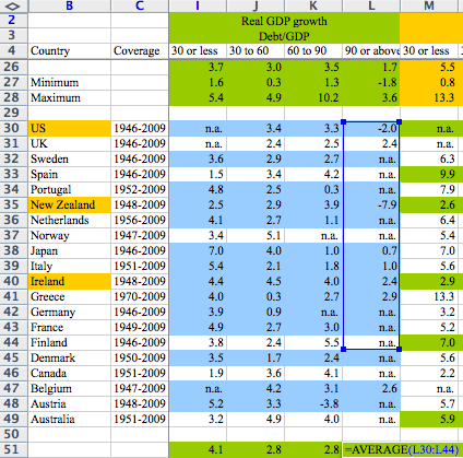
As if to illustrate LeVeque’s point, major news outlets report on a story about a reproducibility error (Excel bug) discovered in the famous politically-influential paper by economists Reinhart and Rogoff:
- Reinhart, Rogoff… and Herndon: The student who caught out the profs (BBS News)
- How much unemployment did Reinhart and Rogoff’s arithmetic mistake cause? (Guardian)
- Is the evidence for austerity based on an Excel spreadsheet error? (Washington Post)
The validity of the Reinhart-Rogoff assertion “once debt exceeds 90 percent of GDP, economic growth drops off sharply” continues to be debated by economists, but it is clear now that their data were flawed and that the error would have been discovered much easier if the publication had followed the reproducible-research discipline.
Zooming in Vplot
April 17, 2013 Programs No comments
sfzoom is a simple Tkinter script that allows for interactive zooming when viewing Vplot files generated by sfgrey. The zoomed images are created by windowing the original RSF file and therefore have the highest possible resolution.

Joe Dellinger has a more comprehensive plan for adding interactivity to Vplot graphics.
How can I read and write RSF files in MATLAB?
April 13, 2013 FAQ No comments
- The most straightforward way is to install the MATLAB interface to Madagascar. When installing Madagascar, run
The configure script will try to find and test matlab and mex executibles on your system. If they are not in your PATH, you can specify them with
Install Madagascar as usual, set MATLAB path to $RSFROOT/lib, and you will able to read and write RSF files from MATLAB using rsf_read, rsf_write, and other functions from the Madagascar interface.

- Alternatively, you can try reading binary data using MATLAB functions, as in the following example
% get in=, n1=, and n2= parameters from file.rsf

[stat,in] = unix(‘sfget in parform=n < file.rsf’)

in = strtrim(in)

[stat,n1] = unix(‘sfget n1 parform=n < file.rsf’)

n1 = str2num(n1)

[stat,n2] = unix(‘sfget n2 parform=n < file.rsf’)

n2 = str2num(n2)

% read binary data

fid = fopen(in,‘rb’)

data = fread(fid,n1*n2,‘float32’);

% reshape to 2-D matrix

data = reshape(data,n1,n2);- An even better alternative is to abandone MATLAB in favor of free software, such as GNU Octave, Python with NumPy, Sage, etc. A Python interface to Madagascar is installed by default.