How do I do interactive picking?

June 12, 2014 FAQ No comments

While interactive picking is generally discouraged because of its non-reproducibility, occasionally it might be useful. Using interact= option with xtpen outputs mouse-click coordinates in a text file. However, they are Vplot coordinates, not easily related to physical coordinates of the image. Joe Dellinger has a more comprehensive plan for adding interactivity to Vplot graphics.

sfipick is a simple Tkinter script which allows for interactive picking. The interface is straightforward. Use left-button mouse clicks to add picks, right-button mouse clicks to remove wrong picks, middle-button to drag picks. The picks are written in a plain text file and can be processed later.

See also:

Program of the month: sfeikonal

June 11, 2014 Programs No comments

sfeikonal solves the eikonal equation using the Fast Marching Method. This computation produces first-arrival traveltimes on a fixed grid.

The following example from sep/fmeiko/fmarch shows traveltime contours for a point source inside the SEG/EAGE salt model.

The point source can be specified by its coordinates xshot=, yzhot=, and zshot= (note that the depth coordinate zshot corresponds to the first axis). In a small box around the source, the solution is computed analytically to avoid errors from the point-source singularity. The size of the box can be specified in samples (b1=, b2=, and b3=) or in physical dimensions (br1=, br2=, and br3=). For a plane-wave source instead of a point source, use plane1=y, plane2=y, or plane3=y. The plane is assumed to be aligned with the grid. For computing a traveltime table with multiple sources, the source coordinates can be specified in a file given by shotfile=. The order of accuracy in the finite-difference scheme is specified by order= parameter.

The following plot from sep/fmsec/cvel shows the error difference between the first- and second-order computations in a constant-velocity medium.

sfeikonal computes isotropic traveltimes. For an extension to VTI anisotropy, see sfeikonalvti.

10 previous programs of the month:

Lowrank on a staggered grid

June 2, 2014 Documentation No comments

A new paper is added to the collection of reproducible documents:
Lowrank seismic wave extrapolation on a staggered grid

We propose a new spectral method and a new finite-difference method for seismic wave extrapolation in time. Using staggered temporal and spatial grids, we derive a wave extrapolation operator using a lowrank decomposition for a first-order system of wave equations and design the corresponding finite-difference scheme. The proposed methods extend previously proposed lowrank and lowrank finite-difference wave extrapolation methods from the cases of constant density to those of variable density. Dispersion analysis demonstrates that the proposed methods have high accuracy for a wide wavenumber range and significantly reduce the numerical dispersion. The method of manufactured solutions coupled with mesh refinement is used to verify each method and to compare numerical errors. 2-D synthetic examples demonstrate that the proposed method is highly accurate and stable. The proposed methods can be used for seismic modeling or reverse time migration.

Second working workshop

June 1, 2014 Celebration 2 comments

Registration is open for Madagascar’s Second Working Workshop.

As a reminder, Working Workshops as opposed to “talking workshops” are meetings where the participants work together (possibly divided into pairs or small teams) to develop new software code or to conduct computational experiments addressing a particular problem. The First Working Workshop took place last summer in Austin. This year’s workshop will take place on at Rice University in Houston, Texas, on July 31 – August 2, 2014. The topic of this year’s workshop is parallel and high-performance computing. The objective is

  1. To develop convenient tools for high-performance and parallel computing.
  2. To create new examples of distributed-memory and shared-memory parallel computing.
  3. To explore hardware-accelerated parallel computing (NVIDIA GPU and Intel® Xeon Phi™).

Registration is free by an application is required. If you are interested in participating in this workshop, please fill an application form.

Tutorial on wave propagation

May 30, 2014 Documentation No comments

A new paper is added to the collection of reproducible documents:
Pengliang Yang from Xi’an Jiaotong University contributes A numerical tour of wave propagation

This tutorial is written for beginners as an introduction to basic wave propagation using finite difference method, from acoustic and elastic wave modeling, to reverse time migration and full waveform inversion. Most of the theoretical delineations summarized in this tutorial have been implemented in Madagascar with Matlab, C and CUDA programming, which will benefit readers’ further study.

Erupting Mount St. Helens

May 27, 2014 Examples No comments

The example in rsf/tutorials/sthelens reproduces the analysis by Evan Bianco of the digital elevation data from Mount St. Helens before and after its catastrophic eruption.


Madagascar users are encouraged to try improving the results.

Light Bartlein color palette

May 15, 2014 Examples No comments

The orange-white-purple diverging color palette was suggested in the article

Light, A. and P.J. Bartlein (2004) The end of the rainbow? Color schemes for improved data graphics. EOS Transactions of the American Geophysical Union 85(40):385

Matteo Niccoli recommends it for seismic data as a replacement for the familiar red-white-blue pallete (color=g in Madagascar). Now the Light-Bartlein palette is available to Madagascar plotting programs, such as sfgrey, as color=lb. See the following example from rsf/rsf/sfgrey:

More information:

Program of the month: sfhelicon

May 13, 2014 Programs No comments

sfhelicon performs multidimensional convolution and inverse convolution (recursive filtering) using the helix transform.

The theory behind helical convolution is explained by Jon Claerbout in the paper

Claerbout, J., 1998, Multidimensional recursive filters via a helix: Geophysics, 63, 1532-1541

and in the corresponding chapter in his book Image Estimation by Example. The following example from gee/hlx/helicon illustrates inverse convolution on a helix.

sfhelicon works in N dimensions. The filter for is supplied by filt= parameter, which points to a real-valued RSF file with filter coefficents. The filter lags on a helix can be stored in a separate integer-value RSF file specified wih lag= parameter (which can be optionally contained inside the file with filter coefficients). The dimensions used for specifying the filter lags are not necessarily the same as the dimensions of the input data and can be specified with n= parameter (which can be optionally contained inside the file with filter lags).

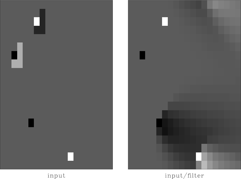
The choice between forward and inverse convolution is controlled by div= parameter. The adjoint flag is supplied by adj= parameter. The following figure illustrates the act of the adjoint convolution and inverse convolution on a helix.

For an example of least-squares inversion with sfhelicon using the conjugate-gradient algorithm, see the documentation for sfconjgrad.

10 previous programs of the month:

madagascar-1.6 released

May 9, 2014 Celebration No comments

The 1.6 stable release features fifteen new reproducible papers and multiple other enhancements including the addition of the seismic migration gallery.

According to the SourceForge statistics, the previous 1.5 stable distribution has been downloaded more than 5,000 times. The record number of downloads in September 2013 is probably due to the fact that Madagascar is being used for teaching at different universities. The top country (with 40% of all downloads) was China, followed by the US, Brazil, Mexico, and Australia.

According to Ohloh.net, the year before the 1.6 release was the period of a high development activity, with 41 contributors (up 41% compared to the previous year) making 1,762 commits to the repository. Ohloh.net says that Madagascar “has a well established, mature codebase maintained by a very large development team with stable year-over-year commits” and estimated 201 man-years of effort.

IWAVE update

April 28, 2014 Documentation No comments

The IWAVE package included in Madagascar went through a significant redesign. The current version is explained in the paper IWAVE Structure and Basic Use Cases by Bill Symes.

The IWAVE control structure facilitates construction of wave simulators with flexible specification of input and output. This document describes synthesis of seismograms and wavefield movies from initial data and from single and multiple sources (right-hand sides), and linearized (“Born”) and linearized adjoint (reverse time migration) modeling. The choice of physical model and simulation method – constant density acoustics with Dirichlet boundary conditions and (2,2k) finite difference schemes – is the simplest possible, but the framework accommodates any regularly gridded stencil-based discretization of arbitrary wave physics in the same way.