Madagascar Development Blog » 2013

Madagascar paper

November 21, 2013 Links No comments

A paper describing Madagascar has been published in the Journal of Open Research Software (JORS), a new peer-reviewed open-access journal, which features papers describing research software with high reuse potential.

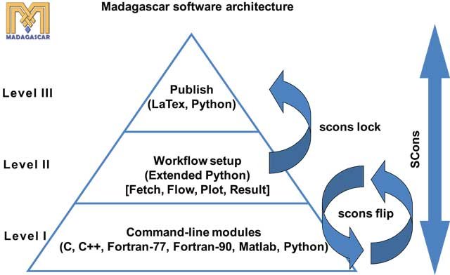
This paper should become a standard reference for those who use Madagascar in their research and wish to reference it in scientific publications. Following a recommendation of Robin Wilson, a file called CITATION.txt is placed in the top Madagascar directory to provide reference information. Here are the current contents of this file:

Fomel, S., Sava, P., Vlad, I., Liu, Y. and Bashkardin, V. 2013. Madagascar:
open-source software project for multidimensional data analysis and
reproducible computational experiments. Journal of Open Research
Software 1(1):e8, DOI: http://dx.doi.org/10.5334/jors.ag

@Article{m8r,
  author = {S. Fomel and P. Sava and I. Vlad and Y. Liu and
                 V. Bashkardin},
  title = {Madagascar: open-source software project for
              multidimensional data analysis and reproducible 
              computational experiments},
  journal =      {Journal of Open Research Software},
  year =      2013,
  volume =      1,
  number =      1,
  pages =      {e8},
  doi =          {http://dx.doi.org/10.5334/jors.ag}}

It is hard to give proper credit to everyone who contributed to such as collaborative project, as Madagascar. Even the smallest contribution can be crucially important. The five authors of the paper are the five most active all-time contributors to Madagascar by the number of commits to the repository at the time of the paper submission.

Geophysical Image Estimation by Example

November 18, 2013 Documentation No comments

Inspired by projects such as the Khan Academy, Jon Claerbout is recording short videos narrating his book, Geophysical Image Estimation by Example. You can reproduce computational examples from the book (translated from Ratfor to C) by following its Madagascar version.

3-D random noise attenuation using f-x-y NRNA

November 13, 2013 Documentation No comments

A new paper is added to the collection of reproducible documents:
Noncausal f-x-y regularized nonstationary prediction filtering for random noise attenuation on 3D seismic data

Seismic noise attenuation is very important for seismic data analysis and interpretation, especially for 3D seismic data. In this paper, we propose a novel method for 3D seismic random noise attenuation by applying noncausal regularized nonstationary autoregression (NRNA) in f-x-y domain. The proposed method, 3D NRNA (f-x-y domain) is the extended version of 2D NRNA (f-x domain). f-x-y NRNA can adaptively estimate seismic events of which slopes vary in 3D space. The key idea of this paper is to consider that the central trace can be predicted by all around this trace from all directions in 3D seismic cube, while the 2D f-x NRNA just considers the middle trace can be predicted by adjacent traces along one space direction. 3D f-x-y NRNA uses more information from circumjacent traces than 2D f-x NRNA to estimate signals. Shaping regularization technology guarantees the nonstationary autoregression problem can be realizable in mathematics with high computational efficiency. Synthetic and field data examples demonstrate that, compared with f-x NRNA method, f-x-y NRNA can be more effective in suppressing random noise and improve trace-by-trace consistency, which are useful in conjunction with interactive interpretation and auto-picking tools such as automatic event tracking.

Random noise attenuation using f-x RNA

November 12, 2013 Documentation No comments

A new paper is added to the collection of reproducible documents:
Random noise attenuation using f-x regularized nonstationary autoregression

We propose a novel method for random noise attenuation in seismic data by applying regularized nonstationary autoregression (RNA) in frequency-space (f-x) domain. The method adaptively predicts the signal with spatial changes in dip or amplitude using f-x RNA. The key idea is to overcome the assumption of linearity and stationarity of the signal in conventional f-x domain prediction technique. The conventional f-x domain prediction technique uses short temporal and spatial analysis windows to cope with the nonstationary of the seismic data. The proposed method does not require windowing strategies in spatial direction. We implement the algorithm by iterated scheme using conjugate gradient method. We constrain the coefficients of nonstationary autoregression (NA) to be smooth along space and frequency in f-x domain. The shaping regularization in least square inversion controls the smoothness of the coefficients of f-x RNA. There are two key parameters in the proposed method: filter length and radius of shaping operator. Synthetic and field data examples demonstrate that, compared with f-x domain and time-space (t-x) domain prediction methods, f-x RNA can be more effective in suppressing random noise and preserving the signals, especially for complex geological structure.

This paper is the first direct contribution from China University of Petroleum (Beijing).

Continuous integration and reproducibility

November 11, 2013 Systems No comments

Continuous Integration (CI) is a technique in software engineering, usually described as one of the common techniques in extreme programming (XP). CI implies maintaining a shared code repository, where developers contribute frequently (possibly several times per day), and an automated build system that includes testing scripts.

Using a CI tool, such as TeamCity, it is easy to implement CI for Madagascar, which includes both compilation tests and reproducibility tests. One of the computers at the University of Texas at Austin has been dedicated to such testing and has helped to detect several bugs and reproducibility problems. You can subscribe to testing reports using the RSS feed. To implement similar testing on your own computer, install TeamCity and configure it as follows:

1. Configure Version Control Settings to connect to the Madagascar Subversion repository.

2. Configure Build Step to use a command-line script such as the following:

./configure --prefix=/tmp/rsfroot 
make install 
source env.sh 
export RSFFIGS=$RSFROOT/share/madagascar/figs 
cd book 
scons test

3. Go out for a cup of coffee and come back to check the results of testing. On a CI server, the run of the “compile & test” script is triggered every time somebody commits a new change to the repository.

4. Fix detected problems and commit your changes back to the repository to continue the integration loop.

Adopting the technique of Continuous Integration, in combination with reproducibility testing, provides a robust development environment with well-debugged code and continuously-maintained reproducible examples. It should encourage an active participation of the Madagascar development community.

Program of the month: sfremap1

November 3, 2013 Programs No comments

sfremap1 interpolates the input data to a different grid along the first axis. Here is an elementary example: making some data and interpolating it to a denser grid:

bash$ sfmath n1=5 o1=0 d1=1 output=x1 | sfdisfil 
0: 0 1 2 3 4 
bash$ sfmath n1=5 o1=0 d1=1 output=x1 | sfremap1 n1=10 d1=0.5 | sfdisfil 
0: 0 0.5 1 1.5 2 
5: 2.5 3 3.5 4 4.5

sfremap1 uses ENO (essentially non-oscillatory) interpolation to prevent oscillations when interpolating discontinuous data:

bash$ sergey$ sfspike n1=10 o1=0 d1=1 k1=6 | sfcausint | sfdisfil 
0: 0 0 0 0 0 
5: 1 1 1 1 1 
bash$ sfspike n1=10 o1=0 d1=1 k1=6 | sfcausint | sfremap1 n1=20 d1=0.5 | sfdisfil 
0: 0 0 0 0 0 
5: 0 0 0 0 0.5 
10: 1 1 1 1 1 
15: 1 1 1 1 1

The ENO algorithm is described by Harten et al. (1987) and Shu and Osher (1988):

A. Harten, B. Engquist, S. Osher, and S. R. Chakravarthy, 1987, Uniformly high order accurate essentially non-oscillatory schemes, III: Journal of Computational Physics, 71(2), 231-303.

C. W. Shu and S. Osher, 1988, Efficient implementation of essentially non-oscillatory shock-capturing schemes: Journal of Computational Physics, 77(2), 439-471.

The interpolation order is controlled by the order= parameter, order=2 corresponds to linear interpolation, the default is order=3. The output grid can be specified either by n1=, o1=, d1= parameters or by providing an example file with the desired grid in pattern= parameter. Here is an example:

bash$ sfmath n1=5 o1=0 d1=1 output=x1 > data.rsf
bash$ sfspike n1=10 d1=0.5 > other.rsf
bash$ < data.rsf sfremap1 pattern=other.rsf | sfdisfil
   0:             0          0.5            1          1.5            2
   5:           2.5            3          3.5            4          4.5

For an alternative method (cubic spline interpolation), see sfspline.

Month: November 2013