A 2-D Modeling experiment using SConstruct

from rsf.proj import *

Flow('vel0',None,
     	'''
     	math output=1.6 n1=50 n2=200 d1=0.005 d2=0.005
     	label1=x1 unit1=km label2=x2 unit2=km 
     	''')

Flow('vel1',None,
     	'''
     	math output=1.8 n1=50 n2=200 d1=0.005 d2=0.005
     	label1=x1 unit1=km label2=x2 unit2=km 
     	''')
Flow('vel2',None,
     	'''
     	math output=2.0 n1=100 n2=200 d1=0.005 d2=0.005
     	label1=x1 unit1=km label2=x2 unit2=km 
     	''')
Flow('vel',['vel0','vel1','vel2'], 'cat axis=1 ${SOURCES[1:3]}')

Result('vel',
       '''
       grey title="velocity model: 3 layers" 
       color=j scalebar=y bartype=v
       ''')

Flow('shots','vel',
	'''
	modeling2d nt=1100 dt=0.001 ns=10 ng=200	
	sxbeg=5 szbeg=2 jsx=20 jsz=0 
	gxbeg=0 gzbeg=3 jgx=1 jgz=0 	
	''')

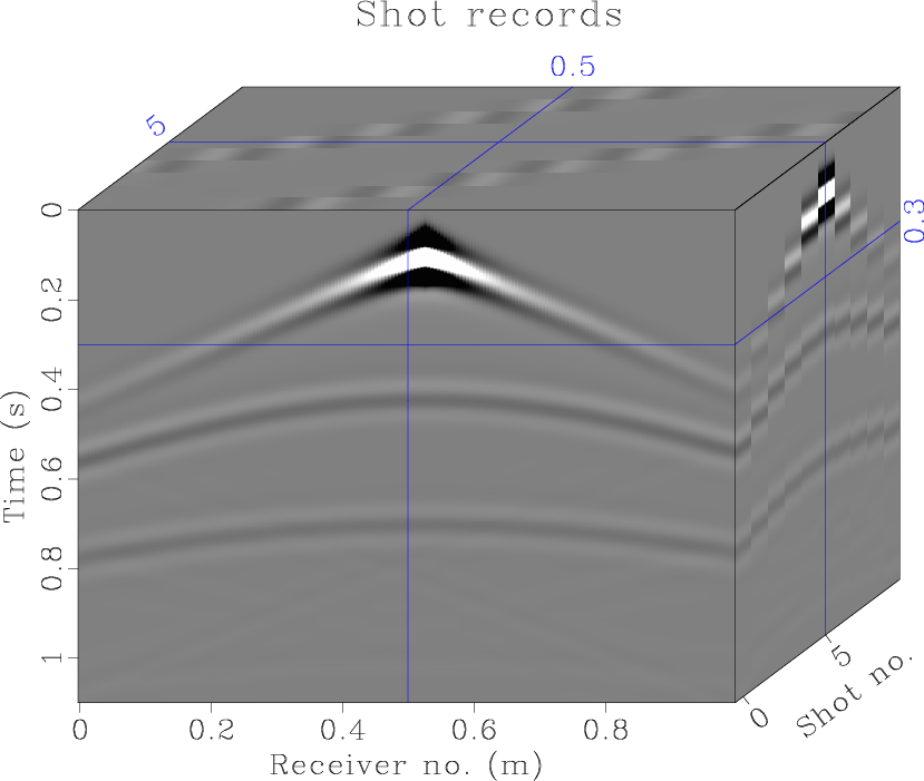
Result('shots',
	'''
       byte allpos=n gainpanel=all |
       grey3 flat=n frame1=300 frame2=100 frame3=5 
       label1=Time unit1=s
       label2="Receiver no." label3="Shot no."
       title="Shot records" point1=0.8 point2=0.8
	''')

Plot('shots','grey title=Shots',view=1)

#use sfwindow to select 5-th shot and display it using sfgrey


End()

We obtain the velocity model in Figure 1 and the shot gathers in Figure 2. To have a look at the movie by looping over each shot gather, run scons.


shots Figure 2. Shot gather