RTM using effective boundary saving: A staggered grid GPU implementation

Effective boundary for staggered grid finite difference

The limitation of boundary saving strategy proposed in Dussaud et al. (2008) is that only regular grid finite difference scheme is considered in RTM. In the case of staggered grid, half grid points are employed to obtain higher accuracy for finite difference. Recursion from time $k$ to $k+1$ (or $k-1$ ) may not be realized with ease due to the Laplacian operator, which involves the second derivative. An effective approach is to split Eq. (1) into several first derivative equations or combinations of first derivative and second derivative equations. The first derivative is defined as

$$\partial_u f=\frac{1}{\Delta u}\left( \sum_{i=1}^{N} c_i(f[u+i\Delta u/2]-f[u-i\Delta u/2])\right), u=z,x$$ (7)

where the finite difference coefficients are listed in Table 2.

Table 2: Finite difference coefficients for staggered grid (Order-$2N$ )

$i$	1	2	3	4
$N=1$	1
$N=2$	1.125	-0.0416667
$N=3$	1.171875	-0.0651041667	0.0046875
$N=4$	1.1962890625	-0.079752604167	0.0095703125	-0.000697544642857

The use of half grid points in staggered grid makes the effective boundary a little different from that in regular grid. To begin with, we define some intermediate auxiliary variables: $Ax:=\partial_x p$ , $Az:=\partial_z p$ , $Px:=\partial_x Ax$ and $Pz:=\partial_z Az$ . Thus the acoustic wave equation reads

$$\left\{ \begin{split}&\frac{\partial^2 p}{\partial t^2}=v^2\lef... ...tial_z Az\\ &Ax=\partial_x p, Az=\partial_z p \end{split} \right.$$ (8)

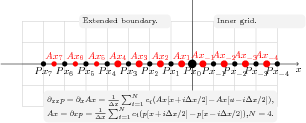
It implies that we have to conduct 2 finite difference steps (one for $Ax$ and $Az$ and the other for $Px$ and $Pz$ ) to compute the Laplacian in one step of time marching. Take 8-th order ($2N=8$ ) finite difference in $x$ dimension for example. As can be seen from Figure 4, computing $\partial _{xx}$ at $Px_0$ needs the correct values at $Ax_4$ ,$Ax_3$ ,$Ax_2$ ,$Ax_1$ in the boundary; computing $Ax_1$ ,$Ax_2$ ,$Ax_3$ ,$Ax_4$ needs the correct values at $Px_4$ ,$Px_5$ ,$Px_6$ ,$Px_7$ in the boundary. An intuitive approach is saving $N$ points of $Ax$ ( $Ax_1,\ldots,Ax_4$ ) and $N$ points of $Px$ ( $Px_4, \ldots, Px_7$ ). The saving procedure guarantees the correctness of these points in the wavefield. Another possible approach is just saving the $2N-1$ points of $Px$ ( $Px_1,\ldots, Px_7$ ). In this way, the values of $Ax_1,\ldots,Ax_4$ can be correctly obtained from the calculation of the first derivative. The latter method is preferable because it is much easier for implementation while requiring less points. 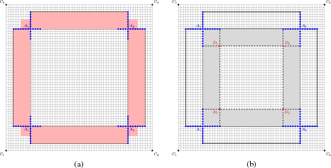Speaking two dimensionally, some points in the four corners at in $B_1B_2B_3B_4$ of Figure 1 may be still necessary to store, as shown in Figure 5a. The reason is that you are working with Laplacian, not second derivative in one dimension. Again, we switch our boundary saving part from out of $A_1A_2A_3A_4$ to $A_1A_2A_3A_4\backslash D_1D_2D_3D_4$ . Less grid points are required to guarantee correct reconstruction while points in the corner are no longer needed. Therefore, the proposed effective boundary for staggered finite difference needs $2N-1$ points to be saved on each side, see Figure 5b.

fig4
Figure 4. $2N$ -th order staggered grid finite difference: correct backward propagation needs $2N-1$ points on one side. For $N=4$ , computing $\partial _{xx}$ at $Px_0$ needs the correct values at $Ax_4$ , $Ax_3$ , $Ax_2$ , $Ax_1$ in the boundary; computing $Ax_4$ ,$Ax_3$ , $Ax_2$ , $Ax_1$ needs the correct values at $Px_4$ , $Px_5$ , $Px_6$ , $Px_7$ in the boundary. Thus, $2N-1=7$ points in boundary zone is required to guarantee the correctness of the inner wavefield.

fig5
Figure 5. A 2-D sketch of required points for boundary saving for staggered grid finite difference: (a) Saving the points outside the model (red region). (b) Effective boundary, saving the points inside the model zone (gray region).

RTM using effective boundary saving: A staggered grid GPU implementation