Deblending in common-receiver domain

Next: Deblending in time-midpoint-offset (TMO) Up: Examples Previous: Examples

Deblending in common-receiver domain

The first example is a synthetic common-receiver gather (CRG). The peak frequency is 30 Hz. The temporal and spatial samplings are 4 ms and 10 m, respectively. There are 512 time samples in this data and there are 256 traces in this data that correspond to 256 different shots. I blended it with another CRG using the random dithering method described by Chen et al. (2014). Being concise, I don't display the other CRG. The unblended and blended data are shown in Figures 4a and 4b, respectively. I used MF and SVMF to denoise the blended data (Figure 4b); I then computed their corresponding noise sections (difference between the blended and deblended sections). The deblending results are shown in Figure 5. While the general deblending effects were similar, it is clear that MF caused much greater loss of energy in the noise sections (see Figures 5c and 5d) than SVMF. The initial filter length for this example is set to be 7. The increments/decrements

are chosen as the default values. Figure 1a shows the map of SR. Figure 1c shows the map of variable filter length for the whole profile. From the scalebar of the map, we can see that the filter length is chosen by the proposed criterion from 3 points to 11 points. By comparing the SR with the different threshold, I was able to identify the signal event and then squeeze the filter length to a safe level: 3 points. For those points which I defined as noise points, the filter length was stretched to the most dangerous level: 11 points.

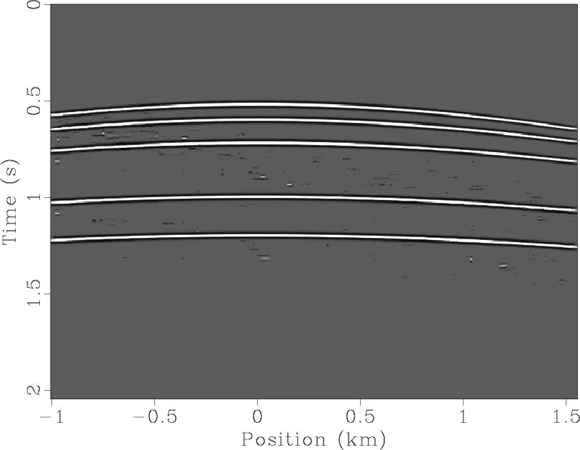
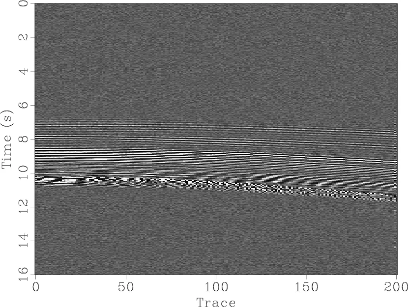
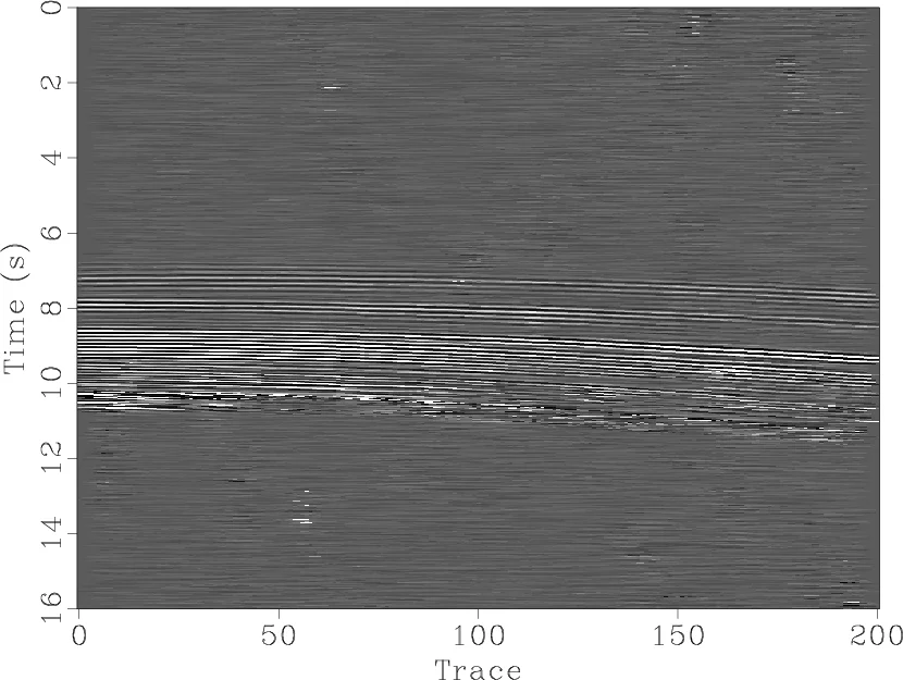
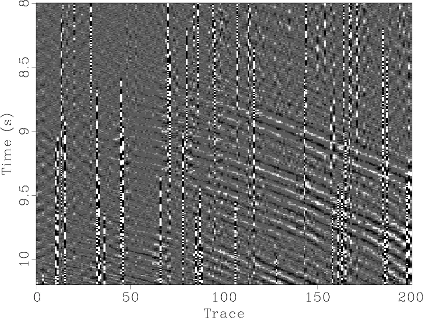
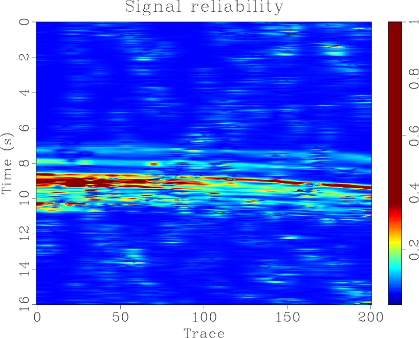
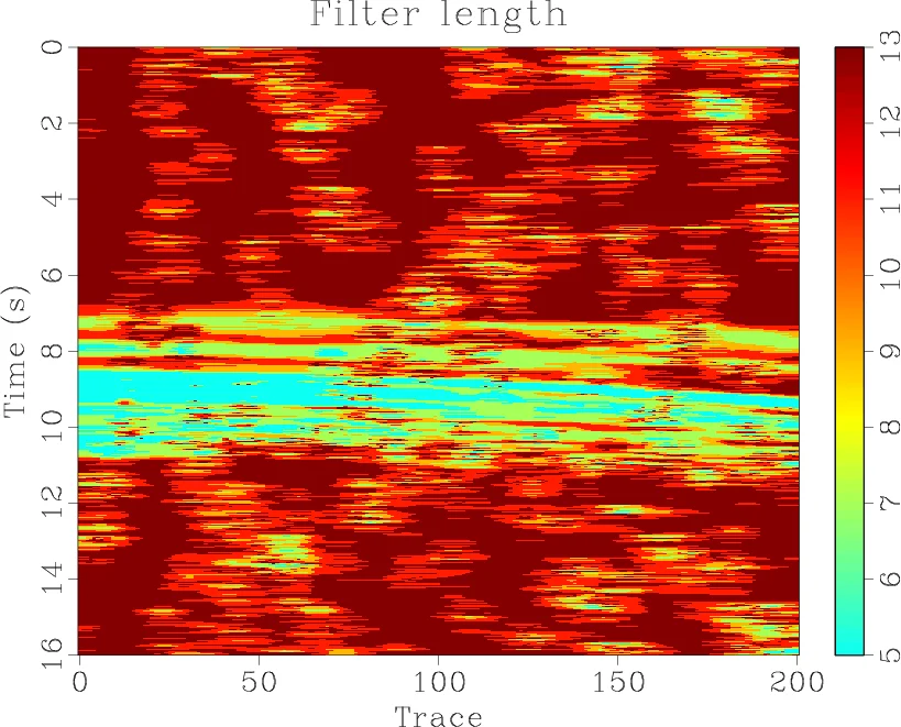
The second example is a marine-field CRG. The temporal sampling is 4 ms. There are 4001 time samples and 201 traces in this CRG. I used the same blending approach as in the first example. The unblended and blended data are shown in Figures 6a and 6b. While both MF and SVMF were able to effectively remove most of the strong spike-like blending noise, SVMF resulted in a much better preservation of the useful signal. The deblending results of MF and SVMF and their corresponding noise sections are shown in Figure 7. For better comparison, two zoomed sections corresponding to the two frame boxes shown in Figure 7 are shown in Figure 8. SVMF clearly causes less loss of useful signal. The initial filter length for this example is set to be 9. The increments/decrements are chosen as the default values. The maps of SR and variable filter length are shown in Figures 9a and 9b. As indicated by the scalebar of the maps, filter length ranged from 5 points to 11 points.


data1,datas Figure 4. Synthetic data examples. (a) Unblended common-receiver-domain data. (b) Blended data.


deblended1mf,deblended1svmf,diff1mf,diff1svmf Figure 5. Demonstration of deblending effects for blended synthetic data. (a)Deblended using MF. (b)Deblended using SVMF. (c)Noise section using MF. (d)Noise section using SVMF.


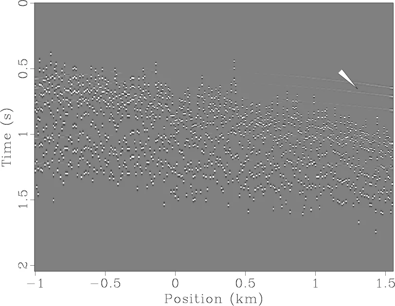
fairunblended2,fairblended2 Figure 6. Marine field data examples. (a) Unblended common-receiver-domain data. (b) Blended data.


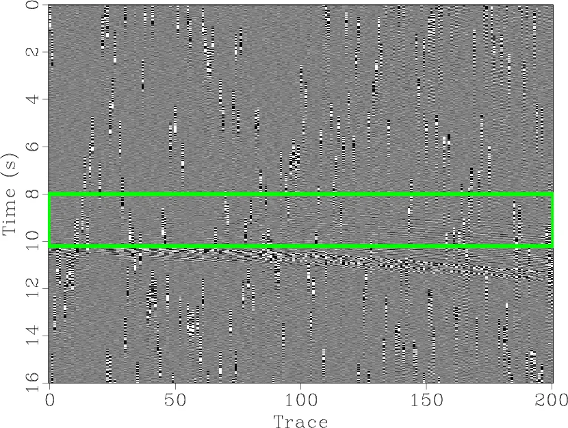
fairdeblended2mf,fairdeblended2svmf,diff2mfframe,diff2svmfframe Figure 7. Demonstration of deblending effects for blended marine field data. (a) Deblended using MF. (b) Deblended using SVMF. (c) Noise section using MF. (d) Noise section using SVMF. The green frame boxes are zoomed in Figure 8 for better comparison.


diff2mfzoom,diff2svmfzoom Figure 8. Zoomed noise sections (corresponding to the two green frame boxes as shown in Figure 7). (a) Zoomed noise section corresponding to MF. (b) Zoomed noise section corresponding to SVMF.


fairsimi2,fairL2 Figure 9. (a) Map of SR for field data. (b) Map of variable filter length for field data.

Next: Deblending in time-midpoint-offset (TMO) Up: Examples Previous: Examples

2015-11-23