|
|
|
|
Nonlinear structure-enhancing filtering using plane-wave prediction |
For the first field-data test, we use a time-migrated seismic
image from a historic Gulf of Mexico dataset
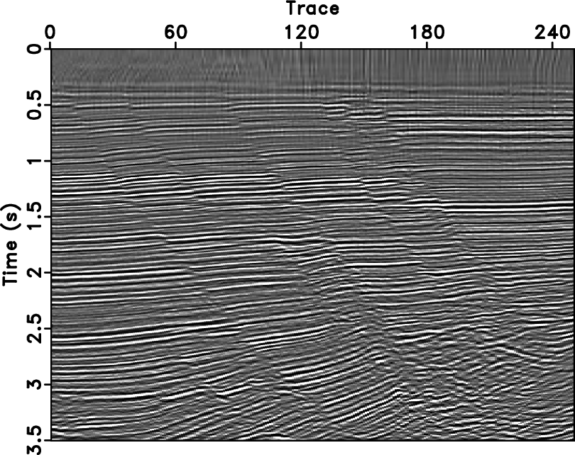
(Claerbout, 2008). The input is shown in
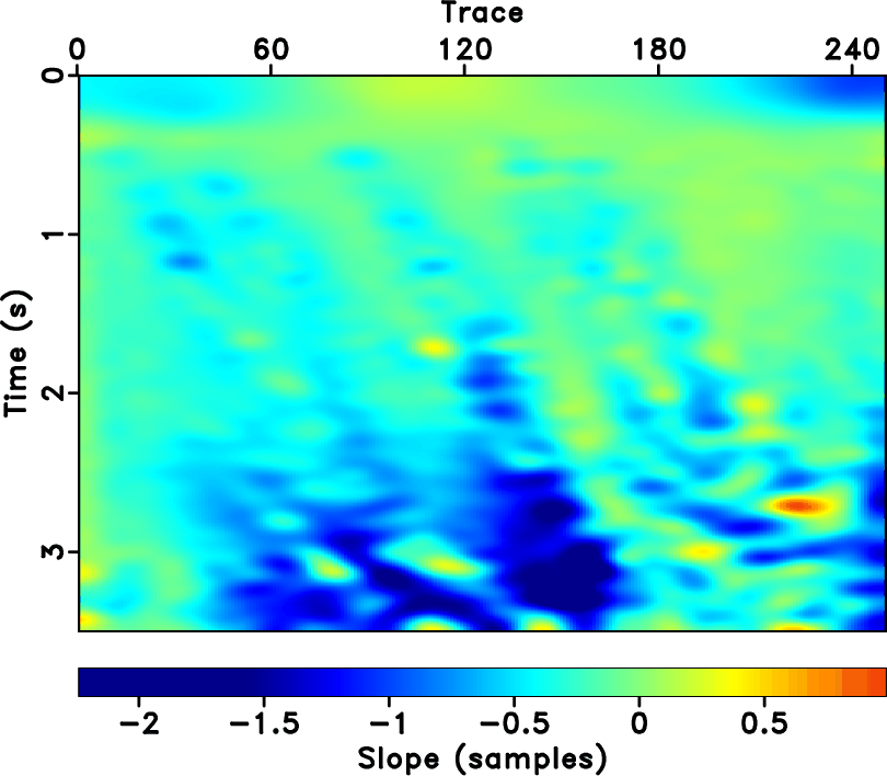
Figure 6a. After estimating the field of local slopes
(Figure 6b), we apply structure prediction to
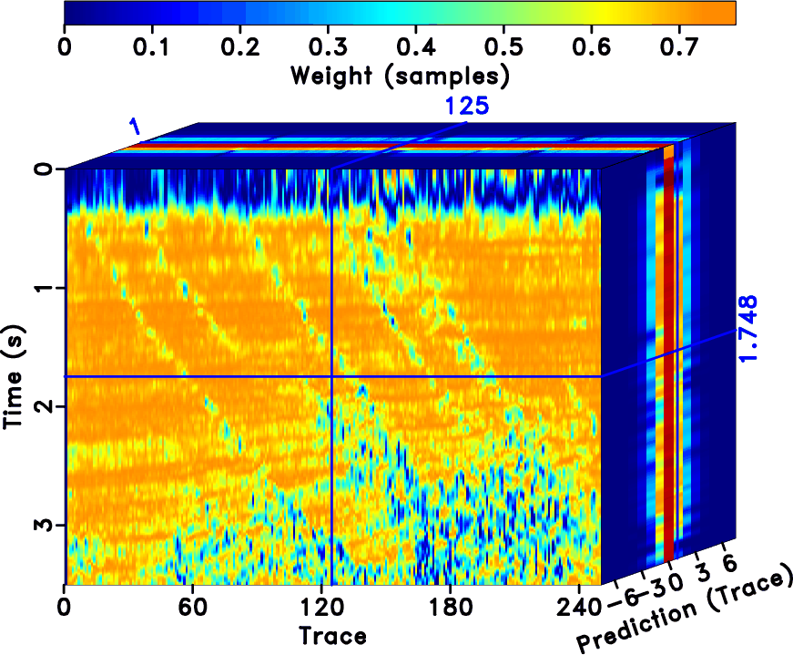
calculate the structural data volume
(Figure 7a), which effectively flattens the
data. As in the synthetic example, the length of the prediction axis
is 15. Next, we apply two different filtering approaches. The first
choice is the similarity-mean filter. We display the product of
Gaussian weights and similarity weights in
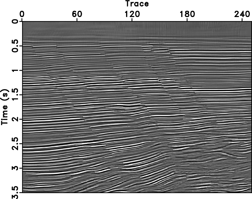
Figure 7b. After applying the similarity-mean
filter, we can get a structure-enhanced image
(Figure 8a): the fault structures are
protected well while noise is removed. Our second choice is an
lower-upper-middle (LUM) filter with parameters ![]() . The enhanced
result is shown in Figure 8b. Similarly
to the similarity-mean filter, the LUM filter highlights locally
continuous reflectors while preserving the geometry of
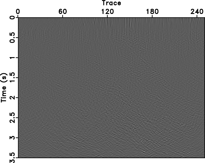
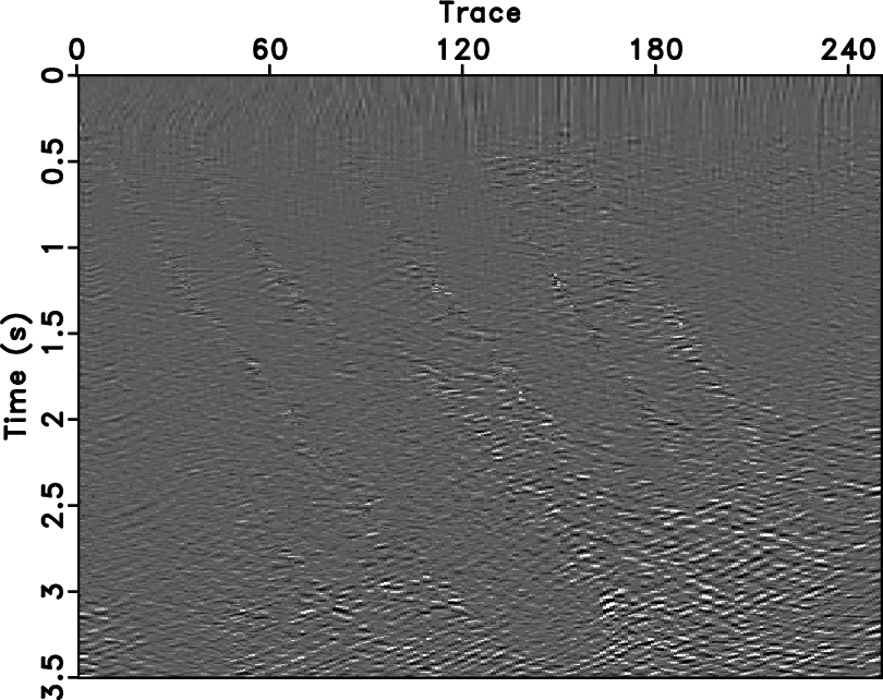
faults. Figure 9 shows the difference sections, in
which the structure-enhancing results using two filtering methods
(Figure 8) are subtracted from the
original data (Figure 6a). After processing, the
coherent events are preserved by both methods. The LUM filter also
removes some short events with crossing dips.
. The enhanced
result is shown in Figure 8b. Similarly
to the similarity-mean filter, the LUM filter highlights locally
continuous reflectors while preserving the geometry of
faults. Figure 9 shows the difference sections, in
which the structure-enhancing results using two filtering methods
(Figure 8) are subtracted from the
original data (Figure 6a). After processing, the
coherent events are preserved by both methods. The LUM filter also
removes some short events with crossing dips.
|
|---|
|
bei,rdip
Figure 6. 2-D field data (a) and local slopes (b). |
|
|

|
|---|
|
rcube,rweight
Figure 7. Predictive data volume (a) and product of Gaussian weights and similarity weights (b). |
|
|

|
|---|
|
rgsimilarstack,rmedian
Figure 8. Structure-enhancing results for image from Figure 6a using similarity-mean filtering (a) and lower-upper-middle (LUM) filtering (b). |
|
|
|
|---|
|
rgdif,rldif
Figure 9. Difference between Figure 6a and structure-enhancing results (Figure 8). Similarity-mean filtering (a) and lower-upper-middle (LUM) filtering (b). |
|
|
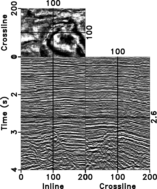
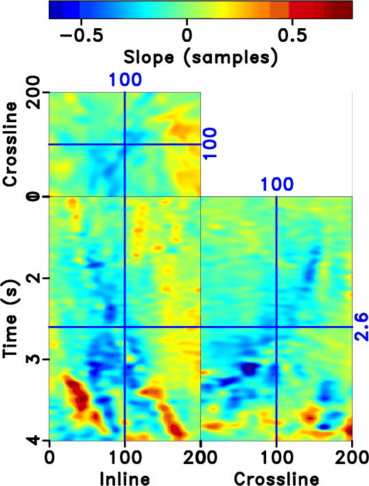
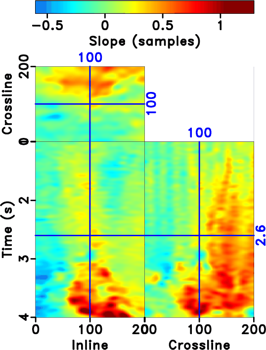
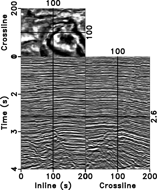
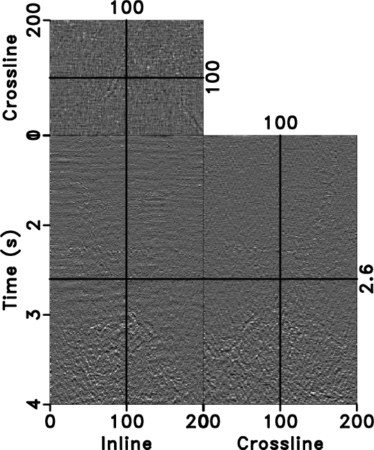
An extension of the method to 3-D is straightforward and follows the 3-D predictive painting construction of Fomel (2008). We use a 3-D field data volume from the Gulf of Mexico to further test our methods (Figure 10). The dataset includes faults having an upside-down cone shape and some amount of random noise. Although variations in amplitude along reflectors can be stratigraphically significant, our goal is to enhance structurally continuous events. We chose a total of 24 prediction traces (2 prediction-step distances around the reference trace), which, with the addition of the original trace, generated a 4-D data volume. The corresponding inline and crossline dips were measured automatically from the image using plane-wave destruction (Figure 11 and 12). Dip sections display different tendencies in inline and crossline directions. Figure 13 and 14 show results of nonlinear structure-enhancing filtering. When processing along the prediction direction, both of our nonlinear filters work well for noise reduction and fault protection. Figure 15 and 16 show the difference sections between the original data (Figure 10) and the structure-enhancing results using two filtering methods (Figure 13 and 14). Similar to the results in the synthetic and 2-D field examples, both methods can protect useful information well.
|
|---|
|
sgr-ori
Figure 10. 3-D image from Gulf of Mexico. |
|
|
|
|---|
|
sgr-dip1
Figure 11. Local inline dip for the 3-D image from Figure 10. |
|
|
|
|---|
|
sgr-dip2
Figure 12. Local crossline dip for the 3-D image from Figure 10. |
|
|

|
|---|
|
sgr-gsstack
Figure 13. Structure-enhancing result using similarity-mean filtering. Compare with Figure 10. |
|
|
|
|---|
|
sgr-lum
Figure 14. Structure-enhancing result using lower-upper-middle (LUM) filtering. Compare with Figure 10. |
|
|

|
|---|
|
sgr-gdif
Figure 15. Difference between Figure 10 and Figure 13. |
|
|
|
|---|
|
sgr-ldif
Figure 16. Difference between Figure 10 and Figure 14. |
|
|
|
|
|
|
Nonlinear structure-enhancing filtering using plane-wave prediction |