|
|
|
|
Relative time seislet transform |
Next: Workflow Up: Theory Previous: RT volume estimation
 and
and
 denote the
  -th and the
  -th
trace, respectively.
-th
trace, respectively.
 is the RT value of the -th trace with the -th trace as
the reference trace, indicating the shift of the -th trace with
respect to the -th trace.
According to equation 9, the prediction of the -th trace
from the -th trace is easily accomplished by simply applying forward
interpolation to the -th trace using corresponding RT values.
In the proposed method, we use equation 9 to define operators
is the RT value of the -th trace with the -th trace as
the reference trace, indicating the shift of the -th trace with
respect to the -th trace.
According to equation 9, the prediction of the -th trace
from the -th trace is easily accomplished by simply applying forward
interpolation to the -th trace using corresponding RT values.
In the proposed method, we use equation 9 to define operators
 in equations 3 and 4 to construct corresponding
prediction and update operators.
In this way, a trace is predicted from a distant trace directly by the
RT attribute instead of the recursive computation used in the PWD-seislet
transform.
Also, because an accurate RT volume stores information about all horizons
and structural discontinuities including faults and unconformities,
predictions of traces around discontinuities using equation
9 are accurate.
Therefore, a better delineation of faults and unconformities can be
achieved.
in equations 3 and 4 to construct corresponding
prediction and update operators.
In this way, a trace is predicted from a distant trace directly by the
RT attribute instead of the recursive computation used in the PWD-seislet
transform.
Also, because an accurate RT volume stores information about all horizons
and structural discontinuities including faults and unconformities,
predictions of traces around discontinuities using equation
9 are accurate.
Therefore, a better delineation of faults and unconformities can be
achieved.
In computing an RT volume, we need to first choose one or multiple reference traces. After computing the RT volume, the RT attribute between any two traces is easily obtained from one RT volume using:
where represents the RT value of the
  -th trace
with the
-th trace
with the  -th trace as the reference trace, and
 is the time
warping (Burnett and Fomel, 2009) of
is the time
warping (Burnett and Fomel, 2009) of
 .
According to equation 10, given the shift information
and
.
According to equation 10, given the shift information
and
 , the shift relationship between the
-th trace and the -th trace can be obtained by applying an inverse
interpolation to
using
.
Then, equation 9 is applied to implement the prediction of the
-th trace from the -th trace.
Therefore, only one RT volume is needed for the proposed implementation of
the seislet transform.
, the shift relationship between the
-th trace and the -th trace can be obtained by applying an inverse
interpolation to
using
.
Then, equation 9 is applied to implement the prediction of the
-th trace from the -th trace.
Therefore, only one RT volume is needed for the proposed implementation of
the seislet transform.
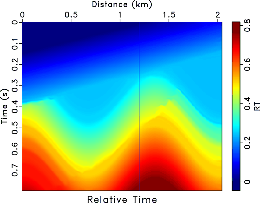
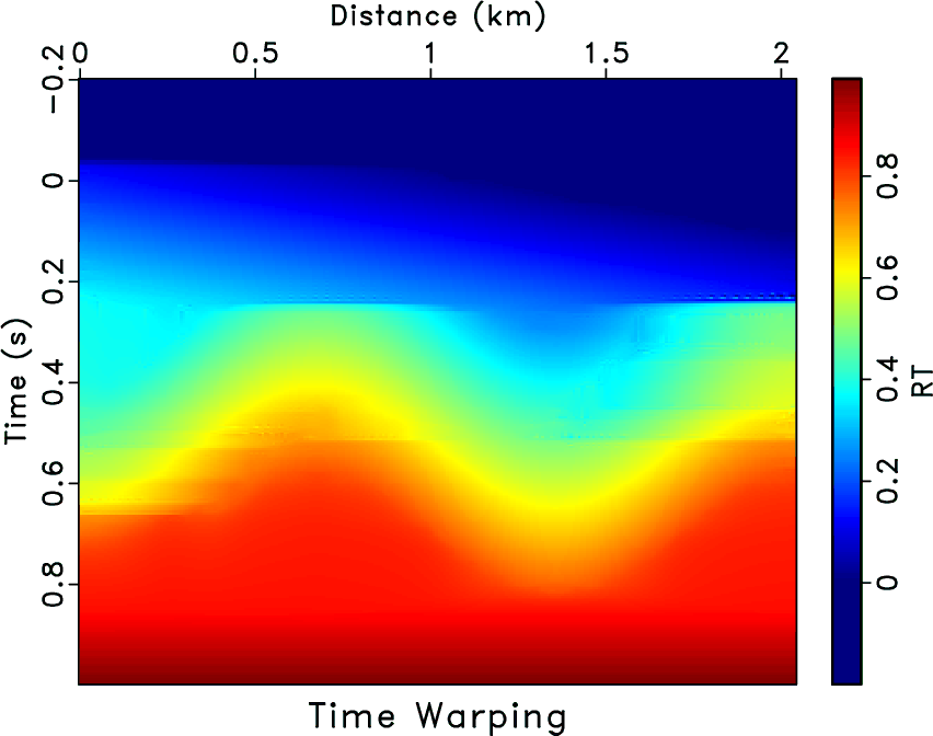
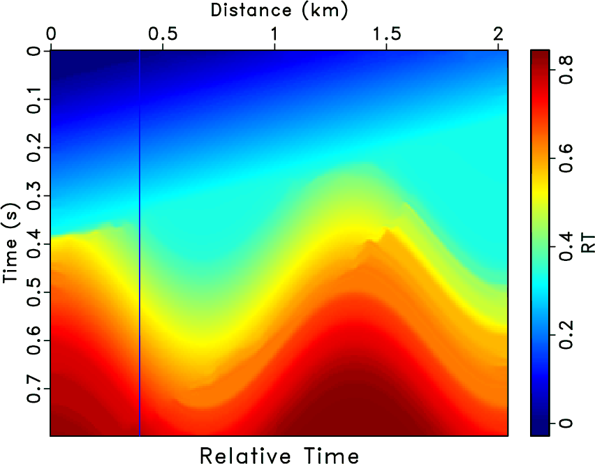
Figure 5 shows an example of
implementing equation 10 to compute an RT volume from another one with
different reference traces.
The RT volume in Figure 5a is obtained by the predictive
painting with the 150th trace as the reference trace.
This RT volume can be represented by
 .
Figure 5b is the time warping of this RT volume.
We extract the 50th trace from Figure 5b, which is denoted by
.
Figure 5b is the time warping of this RT volume.
We extract the 50th trace from Figure 5b, which is denoted by
 .
Then, by implementing equation 10, i.e., inverse interpolating
using the whole RT volume
(
), we can get a new
RT volume, as shown in Figure 5c (
.
Then, by implementing equation 10, i.e., inverse interpolating
using the whole RT volume
(
), we can get a new
RT volume, as shown in Figure 5c (
 ). Here, we use the 50th trace as the reference trace.
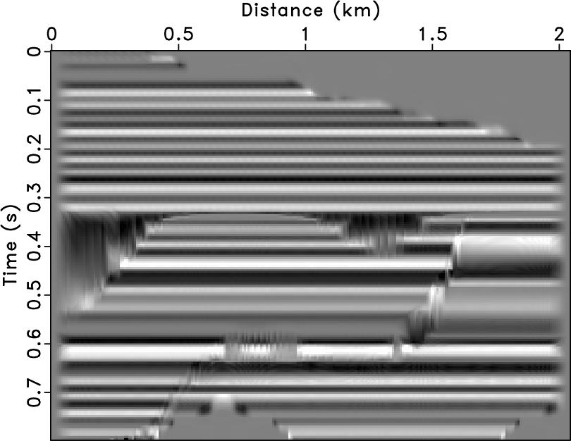
To evaluate the effectiveness of equation 10, RT volumes from
Figure 5c and 5d are used to flatten
Figure 1.
Flattened images are shown in Figure 6.
Small differences between Figure 6a and 6b
indicate that these two RT volumes (Figure 5c
and 5d) contain similar information, which demonstrate
that equation 10 can be used to get the relationship between any two
traces from one single RT volume.
). Here, we use the 50th trace as the reference trace.
To evaluate the effectiveness of equation 10, RT volumes from
Figure 5c and 5d are used to flatten
Figure 1.
Flattened images are shown in Figure 6.
Small differences between Figure 6a and 6b
indicate that these two RT volumes (Figure 5c
and 5d) contain similar information, which demonstrate
that equation 10 can be used to get the relationship between any two
traces from one single RT volume.

|
|---|
|
pick-150,invint,pick-50,pick-50-true
Figure 5. (a) The RT volume obtained by the predictive painting and the reference trace is the 150th trace. (b) Time warping of (a). (c) RT volume obtained by equation 10. (d) The RT volume obtained by the predictive painting and the reference trace is the 50th trace. |
|
|

|
|---|
|
flat1,flat2
Figure 6. Flattened images using RT volumes from (a) Figure 5c and (b) Figure 5d. |
|
|