 |
 |
 |
 | Diffraction imaging and time-migration velocity analysis using oriented velocity continuation |  |
![[pdf]](icons/pdf.png) |
Next: Slope decomposition
Up: Oriented velocity continuation
Previous: Oriented velocity continuation
To adopt the general theory described above to the case of
common-offset 2D oriented velocity continuation, we can substitute
equation (2) into (7), arriving at the
equation
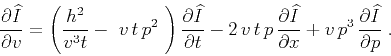 |
(8) |
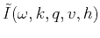
which describes image
propagation in the time-space-slope coordinates rather than the usual
time-space coordinates. After this kind of extrapolation, regular
images can be reconstructed by stacking over offset and slope.
Slope gathers, analogous to dip-angle gathers, can be
extracted before stacking over slope by analyzing  panels for different
image locations
panels for different
image locations  and velocities
  . Measuring flatness of
diffraction events in these gathers provides a means for
estimating migration velocity (Landa et al., 2008; Reshef and Landa, 2009).
. Measuring flatness of
diffraction events in these gathers provides a means for
estimating migration velocity (Landa et al., 2008; Reshef and Landa, 2009).
For practical implementation, the formulation of oriented velocity
continuation can be simplified by employing a stretch from the regular
time coordinate to squared time
 (Fomel, 2003b). According to this
transformation, the Hamilton-Jacobi equation (1) becomes
(Fomel, 2003b). According to this
transformation, the Hamilton-Jacobi equation (1) becomes
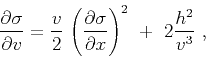 |
(9) |
which leads to the simpler form of the oriented equation
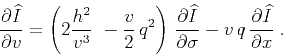 |
(10) |
where  corresponds to
 , and the image is
constructed in
, and the image is
constructed in
 coordinates instead of
  coordinates. Applying the Fourier transform, we
can further transform equation (10) to
coordinates. Applying the Fourier transform, we
can further transform equation (10) to
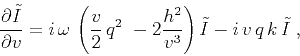 |
(11) |
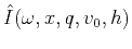
where
 is the double Fourier transform of
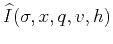 in
in  and .
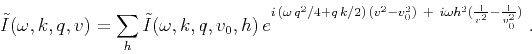
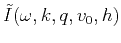
Equation (11) has the analytical solution:
and .
Equation (11) has the analytical solution:
 |
(12) |
where  is a constant non-zero initial migration velocity.
Stacking over offset provides a slope-decomposed formulation for oriented velocity continuation:
 |
(13) |
This derivation suggests the following algorithm for time-domain imaging using common-offset 2D oriented velocity continuation:
- Start with initial time migration with a constant velocity to generate
 .
.
- Apply vertical time stretch to transform from
 to .
to .
- Apply Fourier transform from to
 .
.
- Perform slope decomposition (described in the next section) to generate
 . Note that this operation is parallel in and
  .
.
- Apply Fourier transform from to
 to generate
 . Note that this operation is parallel in and .
- Apply the phase-shift filter from equation (12) to generate
for multiple values of . Note that this operation is data-intensive but parallel in , , and .
- Stack over offset to generate
 .
.
- Apply inverse double Fourier transform to generate
 .
.
- Apply inverse time stretch from to .
- Stack over and extract the slice at time-migration velocity
 to generate the final time-migrated image
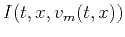 .
.
In order to estimate the velocity , we apply the workflow
described above to diffraction imaging and modify it as follows:
The computational cost associated with determining velocity using oriented velocity continuation is linear with the number of time samples, spatial samples, offsets, velocities, and slopes considered. It is parallel in spatial samples, offsets, velocity, and slope. The cost may then be considered as
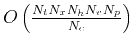 where
where  is the number of cores available.
|
|
|
|
| Diffraction imaging and time-migration velocity analysis using oriented velocity continuation | |
|
Next: Slope decomposition
Up: Oriented velocity continuation
Previous: Oriented velocity continuation
2017-04-20