Analytical solutions in constant velocity

Next: Variable velocity and anisotropy Up: Theory Previous: Theory

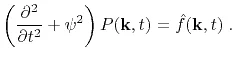
Analytical solutions in constant velocity

When V is constant, after Fourier transform in space, the wave equation takes the form

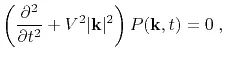$\displaystyle \left( \frac{\partial^2}{\partial t^2} + V^2 \vert\mathbf{k}\vert^2 \right) P(\mathbf{k},t)=0\; ,$

(2)

where $\mathbf{k}$ is the spatial wavenumber and $P(\mathbf{k},t)$ is the spatial Fourier transform of $p(\mathbf{x},t)$ :

$\displaystyle P(\mathbf{k},t) = \frac{1}{(2\pi)^3}\int p(\mathbf{x},t) e^{-i\mathbf{k}\cdot\mathbf{x}}d\mathbf{x}\; .$

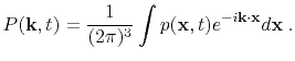(3)

The analytical solution to equation 2 can be expressed as

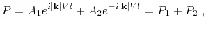$\displaystyle P = A_1 e^{i\vert\mathbf{k}\vert Vt} + A_2 e^{-i\vert\mathbf{k}\vert Vt} = P_1 + P_2 \; ,$

(4)

where

represents the forward-propagating wavefield, i.e., positive frequencies, and

represents the backward-propagating wavefield, i.e., negative frequencies. The time derivative of

has the following form:

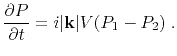$\displaystyle \frac{\partial P}{\partial t}=i\vert\mathbf{k}\vert V(P_1-P_2)\;.$

(5)

Zhang and Zhang (2009) used the Hilbert transform to define an additional function:

$\displaystyle Q(\mathbf{k},t)=\frac{1}{\psi}\frac{\partial P(\mathbf{k},t)}{\partial t}\;,$

(6)

where $Q(\mathbf{k},t)$ is the Hilbert transform of $P(\mathbf{k},t)$ , and $\psi=V\vert\mathbf{k}\vert$ . Combining equations 4, 5 and 6,

and

can be expressed as

$\displaystyle P_1=\frac{1}{2}\left(P - iQ \right) \; ,$			(7)
$\displaystyle P_2=\frac{1}{2}\left(P + iQ \right) \; .$			(8)

Equation 2 can be split into a pair of first-order equations and expressed in the following matrix form:

$\displaystyle \frac{\partial}{\partial t}\left[ \begin{array}{c} P P_t \end{... ...end{array} \right] \; \left[ \begin{array}{c} P P_t \end{array} \right] \; .$

(9)

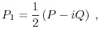
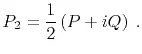
With the help of the Hilbert transform and equations 7 and 8, a more symmetric expression can be achieved:

$\displaystyle \frac{\partial}{\partial t}\left[ \begin{array}{c} P iQ \end{a... ...\end{array} \right] \; \left[ \begin{array}{c} P iQ \end{array} \right] \; .$

(10)

We can further decompose the first matrix on the right-hand side as follows:

$\begin{displaymath}\left[ \begin{array}{cc} 0 & -i\psi \\ -i\psi & 0 \end{ar... ...{array}{cc} 1/2 & -1/2 \\ 1/2 & 1/2 \end{array} \right] \; .\end{displaymath}$

(11)

Substituting equation 11 into equation 10, and using equations 7 and 8, we arrive at:

$\displaystyle \frac{\partial}{\partial t}\left[ \begin{array}{c} P iQ \end{a... ...d{array} \right] \; \left[ \begin{array}{c} P_1 P_2 \end{array} \right] \; .$

(12)

In RTM, only one branch of the total wavefield is needed at one time. The two parts of wave propagation decouple according to

$\displaystyle \frac{\partial}{\partial t}\left[ \begin{array}{c} P_1 P_2 \en... ...d{array} \right] \; \left[ \begin{array}{c} P_1 P_2 \end{array} \right] \; .$

(13)

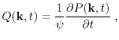
Modeling seismic wave propagation requires the source function. Letting the source function be $f(\mathbf{x},t)$ , wave equation 2 can be rewritten in the following form:

$\displaystyle \left( \frac{\partial^2}{\partial t^2} + \psi^2 \right) P(\mathbf{k},t)=\hat{f}(\mathbf{k},t) \; .$

(14)

Correspondingly, equation 13 becomes:

$\begin{displaymath}\frac{\partial}{\partial t}\left[ \begin{array}{c} P_1 \\ P_2 \end{array} \right]\end{displaymath}$	$\displaystyle =$	$\begin{displaymath}\left[ \begin{array}{cc} 1/2 & -1/2 \\ 1/2 & 1/2 \end{arra... ...}{c} 0 \\ \frac{i}{\psi} \hat{f} \end{array} \right] \right\}\end{displaymath}$	(15)
	$\displaystyle =$	$\begin{displaymath}\left[ \begin{array}{cc} i\psi & 0 \\ 0 & -i\psi \end{arr... ...,\hat{f} \\ \frac{i}{2\psi} \hat{f} \end{array} \right] \; .\end{displaymath}$

The application of operator $-i/2\psi$ can be implemented in either time domain or Fourier domain; it can also be directly incorporated into the definition of source functions. For example, operator $1/\psi$ can be regarded as $(i\omega/\vert\omega\vert) \cdot (1/i\omega)$ , which in the time domain corresponds to cascading the Hilbert-transform with the first-order integration.

In constant velocity, the forward-propagating wavefield away from the source at the next time step $t+\Delta t$ can be expressed as:

$\displaystyle p_1(\mathbf{x},t+\Delta t) = \int P_1(\mathbf{k},t) e^{i [\mathbf{k} \cdot \mathbf{x} + V \vert\mathbf{k}\vert \Delta t]} d\mathbf{k}\;.$

(16)

Next: Variable velocity and anisotropy Up: Theory Previous: Theory

2016-11-16