|
|
|
|
Lowrank finite-differences and lowrank Fourier finite-differences for seismic wave extrapolation in the acoustic approximation |
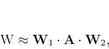
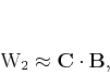
In a matrix notation, the lowrank decomposition problem takes the following form:
Note that ![]() is a matrix related only to wavenumber
is a matrix related only to wavenumber ![]() .
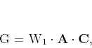
We propose to further decompose it as follows:
.
We propose to further decompose it as follows:
 ,
in which
,
in which
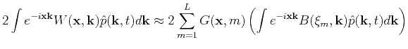
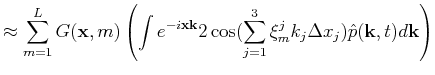
Equation 14 indicates a procedure of finite differences for wave extrapolation: the integer vector,
![]() provides the stencil information, and
provides the stencil information, and
![]() stores the corresponding coefficients.
We call this method lowrank finite differences (LFD)
because the finite-difference coefficients are derived from a lowrank approximation of the mixed-domain propagator matrix.
We expect the derived LFD scheme to accurately propagate seismic-wave components within a wide range of wavenumbers,
which has advantages over conventional finite differences that focus mainly on small wavenumbers.
In comparison with the Fourier-domain approach, the cost is reduced to
stores the corresponding coefficients.
We call this method lowrank finite differences (LFD)
because the finite-difference coefficients are derived from a lowrank approximation of the mixed-domain propagator matrix.
We expect the derived LFD scheme to accurately propagate seismic-wave components within a wide range of wavenumbers,
which has advantages over conventional finite differences that focus mainly on small wavenumbers.
In comparison with the Fourier-domain approach, the cost is reduced to ![]() ,
where
,
where ![]() , as the row size of matrix
, as the row size of matrix ![]() , is related to the order of the scheme.
, is related to the order of the scheme.
![]() can be used to characterize the number of FD coefficients in the LFD scheme, shown in equation 14.
Take the 1-D 10th order LFD as an example, there are 1 center point, 5 left points (
can be used to characterize the number of FD coefficients in the LFD scheme, shown in equation 14.
Take the 1-D 10th order LFD as an example, there are 1 center point, 5 left points (![]() ) and 5 right ones (
) and 5 right ones (![]() ).
So
).
So
![]() , and
, and
![]() .
Thanks to the symmetry of the scheme,
coefficients of
.
Thanks to the symmetry of the scheme,
coefficients of ![]() and
and ![]() are the same, as indicated by equation 14.
As a result, one only needs 6 coefficients:
are the same, as indicated by equation 14.
As a result, one only needs 6 coefficients: ![]() .
.


|
|---|
|
Mexact,Mlrerr,Mapperr,Mfd10err
Figure 1. (a) Wavefield extrapolation matrix for 1-D linearly increasing velocity model. Error of wavefield extrapolation matrix by:(b) lowrank approximation, (c) the 10th-order lowrank FD (d) the 10th-order FD. |
|
|
We use a one-dimentional example shown in Figure 1 to demonstrate the accuracy of the proposed LFD method.
The velocity linearly increases from 1000 to 2275 m/s.
The rank is 3 (![]() ) for lowrank decomposition for this model with 1 ms time step.
The propagator matrix is shown in Figure 1a.
Figure 1b-Figure 1d display the errors corresponding to different approximations.
The error by the 10th-order lowrank finite differences (Figure 1c) appears significantly smaller than that of the 10th-order finite difference (Figure 1d).
Figure 2 displays the middle column of the error matrix. Note that the error of the LFD is significantly closer to zero than that of the FD method.
) for lowrank decomposition for this model with 1 ms time step.
The propagator matrix is shown in Figure 1a.
Figure 1b-Figure 1d display the errors corresponding to different approximations.
The error by the 10th-order lowrank finite differences (Figure 1c) appears significantly smaller than that of the 10th-order finite difference (Figure 1d).
Figure 2 displays the middle column of the error matrix. Note that the error of the LFD is significantly closer to zero than that of the FD method.
|
slicel
Figure 2. Middle column of the error matrix. Solid line: the 10th-order LFD. Dash line: the 10th-order FD. |

|
|---|---|
|
|
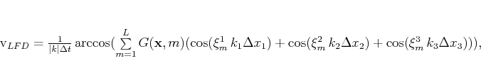
To analyze the accuracy, we let


|
|---|
|
app,fd10
Figure 3. Plot of 1-D dispersion curves for different velocities, |
|
|
|
|
|
|
Lowrank finite-differences and lowrank Fourier finite-differences for seismic wave extrapolation in the acoustic approximation |

![$\displaystyle \approx \sum\limits_{m=1}^L G(\mathbf{x},m) \left[\int e^{-i \mat...
...mits_{j=1}^3{\xi_m^j k_j\Delta x_j}})\hat{p}(\mathbf{k},t) d\mathbf{k} \right].$](img76.png)
![\begin{displaymath}
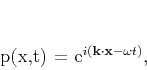
p(\mathbf{x},t+\Delta t) + p(\mathbf{x},t-\Delta t) = \su...
...m=1}^L G(\mathbf{x},m) [p(\mathbf{x}_L,t)+p(\mathbf{x}_R,t)],
\end{displaymath}](img77.png)