|
|
|
|
Predictive painting across faults |
Next: Example for area partition Up: Xue, Wu & Fomel: Previous: Unfaulting method
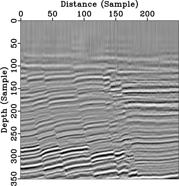
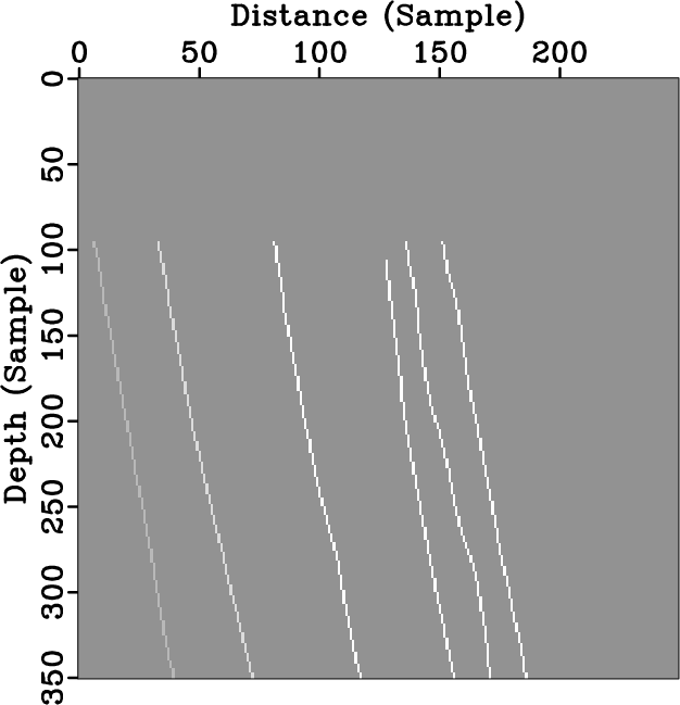
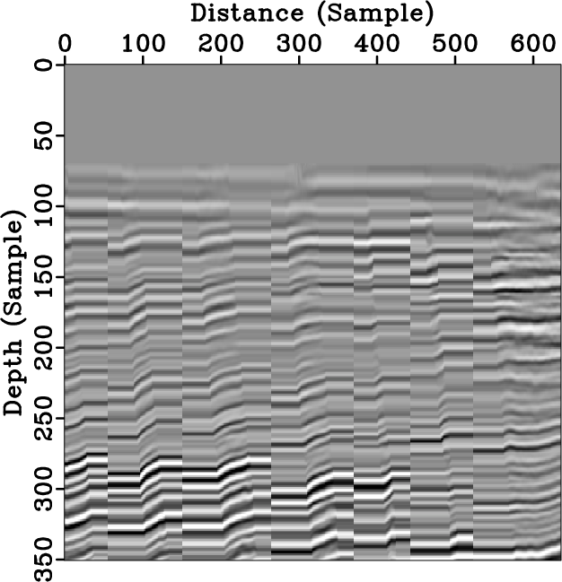
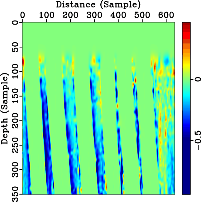
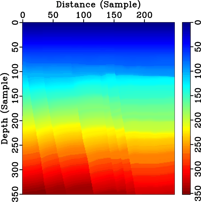
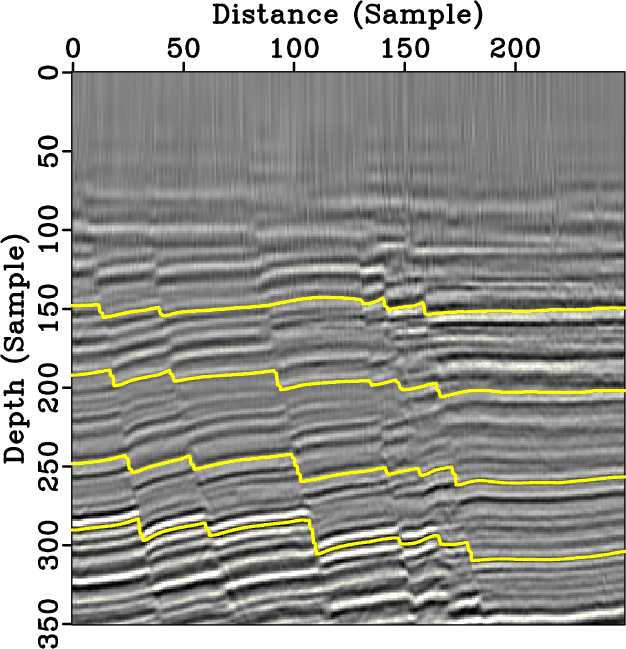
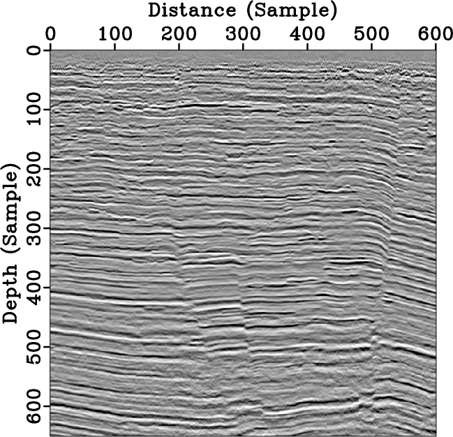
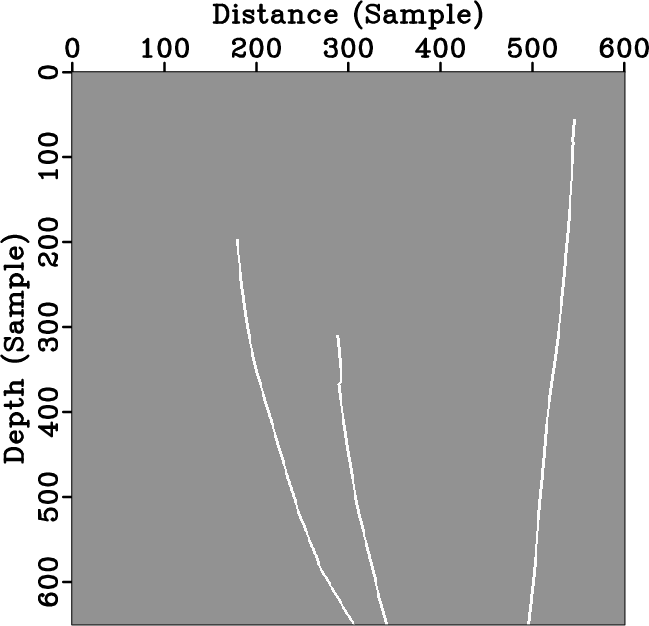
In this section, we use three 2D examples to verify the effectiveness of the proposed three methods. We test an application of predictive painting for horizon picking on all the 2D images. In this application, the depth coordinate is regarded as the reference trace being spread recursively from left to right. The spreading result is referred to as relative geologic time (Stark, 2004), and each contour of it represents a horizon. All the images contain several faults, and we want to correctly pick several horizons using our methods of predictive painting across faults. The fault maps in all the examples are estimated using the method proposed by Wu and Hale (2016).
|
|---|
|
seis,mask,seis2,dip3,paint2,pick2
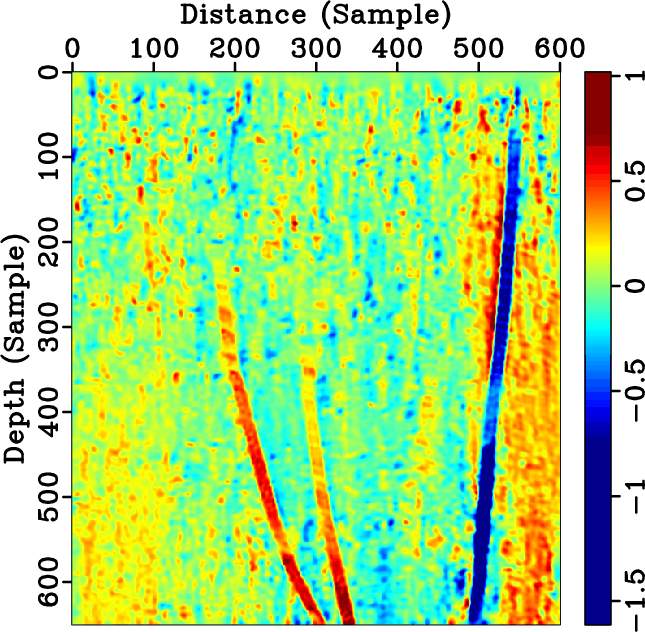
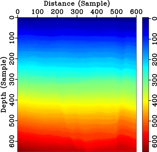
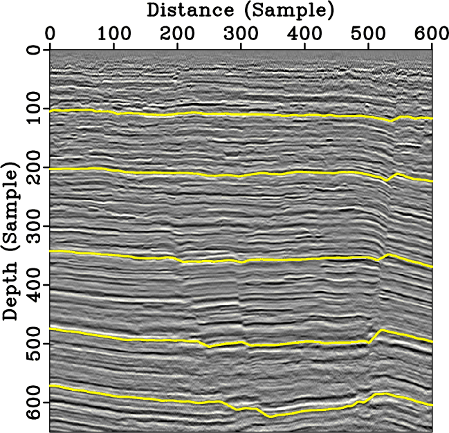
Figure 2. A 2D example for area partition method. (a) Original image; (b) fault mask; (c) new image after area partition and padding with zero slope; (d) dip of the new image (dip around vertical boundaries is set to be zero); (e) final predictive painting result (displayed on the original grid mesh); (f) several automatically picked horizons. |
|
|

|
|---|
|
lseis,lmask,lseis2,ldip2,lpaint2,lpick2
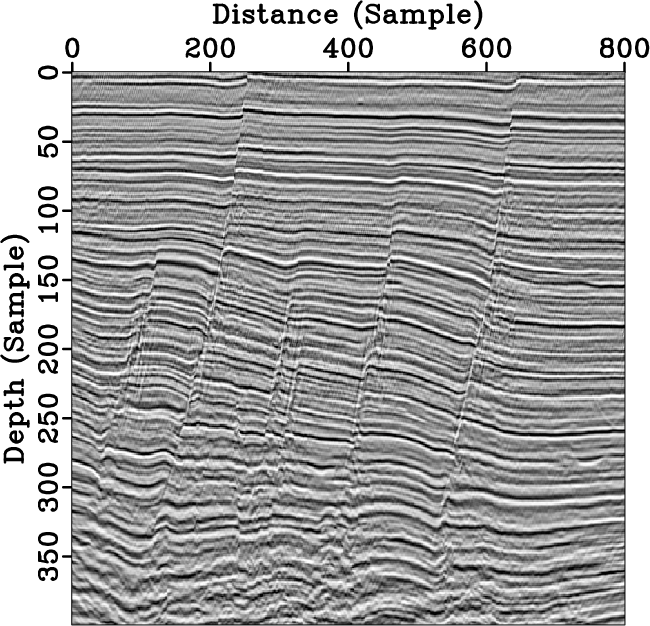
Figure 3. A 2D example for fault-zone replacement method. (a) Original image; (b) fault mask; (c) new image after replacing fault zones with smooth transitions; (d) dip of the new image; (e) predictive painting using dip in Figure 3d; (f) several automatically picked horizons. |
|
|




|
|---|
|
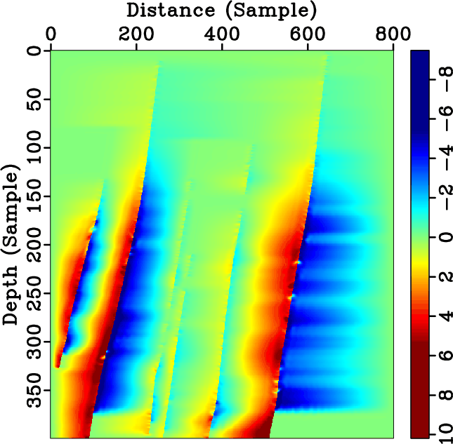
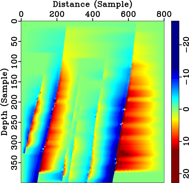
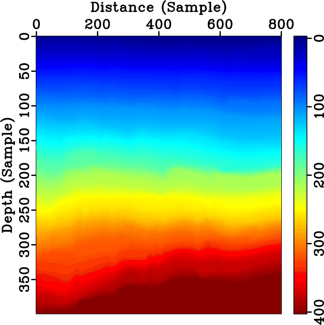
cseis,cmask,cshiftx,cshiftz,cseis22,cpaint2,cpaint3,cpick3
Figure 4. A 2D example for unfaulting method. (a) Original image; (b) fault mask; (c) the horizontal component of the shift vector; (d) the vertical component of the shift vector; (e) new image after undoing faulting of the original image; (f) predictive painting of the unfaulted image; (g) predictive painting of the original image, obtained by faulting the result in Figure 4f; (h) several automatically picked horizons. |
|
|