Finite-difference approach

Next: Fourier approach Up: Numerical velocity continuation in Previous: Numerical velocity continuation in

Finite-difference approach

The differential equation (1) has a mathematical form analogous to that of the 15-degree wave extrapolation equation (Claerbout, 1976). Its finite-difference implementation, first described by Claerbout (1986) and Li (1986), is also analogous to that of the 15-degree equation, except for the variable coefficients. One can write the implicit unconditionally stable finite-difference scheme for the velocity continuation equation in the form

$\begin{displaymath} ({\bf I} + a_{j+1}^{i+1} {\bf T}) {\bf P}_{j+1}^{i+1} - (... ...{i} + ({\bf I} + a_{j}^{i} {\bf T}) {\bf P}_{j}^{i} = 0\;, \end{displaymath}$

(5)

where index

corresponds to the time dimension, index

corresponds to the velocity dimension, ${\bf P}$ is a vector along the midpoint direction, ${\bf I}$ is the identity matrix, ${\bf T}$ represents the finite-difference approximation to the second-derivative operator in midpoint, and $a_{j}^{i} = v_j t_i {\Delta v \Delta t}$ .

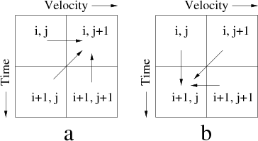
In the two-dimensional case, equation 5 reduces to a tridiagonal system of linear equations, which can be easily inverted. In 3-D, a straightforward extension can be obtained by using either directional splitting or helical schemes (Rickett et al., 1998). The direction of stable propagation is either forward in velocity and backward in time or backward in velocity and forward in time as shown in Figure 1.

vlcfds Figure 1. Finite-difference scheme for the velocity continuation equation. A stable propagation is either forward in velocity and backward in time (a) or backward in velocity and forward in time (b).

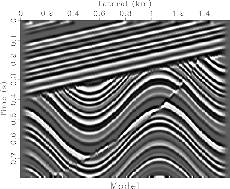
In order to test the performance of the finite-difference velocity continuation method, I use a simple synthetic model from Claerbout (1995). The reflectivity model is shown in Figure 2. It contains several features that challenge the migration performance: dipping beds, unconformity, syncline, anticline, and fault. The velocity is taken to be constant $v=1.5 \mbox{km/s}$ .

mod Figure 2. Synthetic model for testing finite-difference migration by velocity continuation.

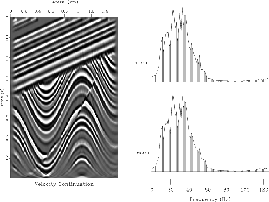
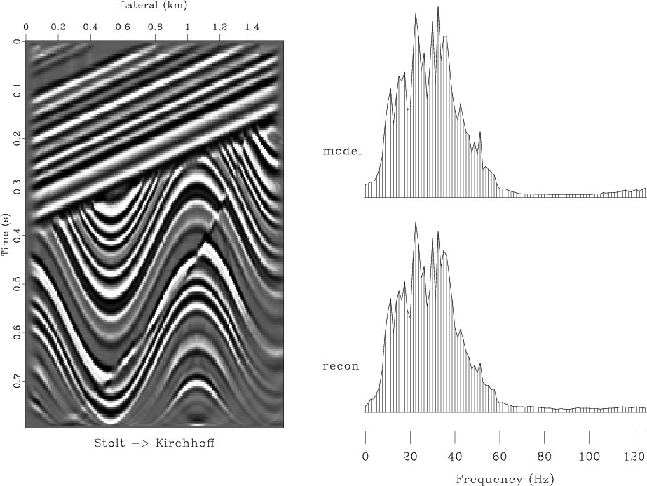
Figures 3-6(b) compare invertability of different migration methods. In all cases, constant-velocity modeling (demigration) was followed by migration with the correct velocity. Figures 3 and 4 show the results of modeling and migration with the Kirchhoff (Schneider, 1978) and - (Stolt, 1978) methods, respectively. These figures should be compared with Figure 5, showing the analogous result of the finite-difference velocity continuation. The comparison reveals a remarkable invertability of velocity continuation, which reconstructs accurately the main features and frequency content of the model. Since the forward operators were different for different migrations, this comparison did not test the migration properties themselves. For such a test, I compare the results of the Kirchhoff and velocity-continuation migrations after Stolt modeling. The result of velocity continuation, shown in Figure 6, is noticeably more accurate than that of the Kirchhoff method.


vlckaa Figure 3. Result of modeling and migration with the Kirchhoff method. Top left plot shows the reconstructed model. Top right plot compares the average amplitude spectrum of the true model with that of the reconstructed image. Bottom left is the reconstruction error. Bottom right is the absolute error in the spectrum.


vlcsto Figure 4. Result of modeling and migration with the Stolt method. Top left plot shows the reconstructed model. Top right plot compares the average amplitude spectrum of the true model with that of the reconstructed image. Bottom left is the reconstruction error. Bottom right is the absolute error in the spectrum.


vlcvel Figure 5. Result of modeling and migration with the finite-difference velocity continuation. Top left plot shows the reconstructed model. Top right plot compares the average amplitude spectrum of the true model with that of the reconstructed image. Bottom left is the reconstruction error. Bottom right is the absolute error in the spectrum.


vlcstk,vlcstv Figure 6. (a) Modeling with Stolt method, migration with the Kirchhoff method. (b) Modeling with Stolt method, migration with the finite-difference velocity continuation. Left plots show the reconstructed models. Right plots show the reconstruction errors.

These tests confirm that finite-difference velocity continuation is an attractive migration method. It possesses remarkable invertability properties, which may be useful in applications that require inversion. While the traditional migration methods transform the data between two completely different domains (data-space and image-space), velocity continuation accomplishes the same transformation by propagating the data in the extended domain along the velocity direction. Inverse propagation restores the original data. According to Li (1986), the computational speed of this method compares favorably with that of Stolt migration. The advantage is apparent for cascaded migration or migration with multiple velocity models. In these cases, the cost of Stolt migration increases in direct proportion to the number of velocity models, while the cost of velocity continuation stays the same.

Next: Fourier approach Up: Numerical velocity continuation in Previous: Numerical velocity continuation in

2013-03-03