Marmousi Model

Finite Difference Modeling

Madagascar can perform finite difference modeling on the Amoco Velocity model. This is done using the function fdmod. The raw velocity model needs to be formatted in a similar fashion to the Model Section of this paper.

For the purposes of this example a shot will be fired at 5 km along the horizontal coordinate and at a depth of 10 meters. Receivers are spread at a depth of 25 meters every 12.5 meters along the entire scope of the model. This long receiver cable is impractical but useful for these purposes. Data is recorded on every receiver at time increments of 1 ms 5000 times resulting in 5 seconds of data. In practice it would be necessary to perform longer running models, but this number of time gates is sufficient for this introduction.

An SConstruct file located within marmousi/fdmod/ properly formats the model and inputs necessary parameters to perform a shot on the Marmousi model. This file is reproduced below in Table 6.

from rsf.proj import *
import fdmod
# Fetch Files from repository
raw=['marmvel.hh','marmsmooth.HH']
for file in raw:
    Fetch(file,"marm")
    if file is 'marmvel.hh':
        d=.004
        fileOut='marmvel'
        t='Velocity Model'
    if file is 'marmsmooth.HH':
        d=.024
        fileOut='marmsmooth'
        t='Smoothed Velocity Model'
# Convert Files to RSF and update headers
    Flow(fileOut,file,'''dd form=native |
        scale rscale=.001 | put
        label1=Depth label2=Position unit1=km unit2=km
        d1=%f d2=%f''' % (d,d))
# Plotting Section
    Result(fileOut,'''window $SOURCE  |
        grey color=I gainpanel=a allpos=y scalebar=y
        title=%s barlabel=kms screenratio=.326
        screenht=3 wheretitle=t labelsz=4 titlesz=6 ''' % t)

# ------------------------------
par = {
    'nt':10000, 'dt':0.00025,'ot':0,'lt':'t','ut':'s',
    'nx':2301, 'ox':0, 'dx':.004, 'lx':'x','ux':'km',
    'nz':751,  'oz':0, 'dz':.004, 'lz':'z','uz':'km',
    'kt':400    # wavelet delay
    }
# add F-D modeling parameters
fdmod.param(par)
# ------------------------------
# wavelet
Flow('wav',None,
         '''spike nsp=1 mag=1 n1=%(nt)d d1=%(dt)g o1=%(ot)g k1=%(kt)d |
         ricker1 frequency=15 | scale axis=123 | 
         put label1=t label2=x label3=y | transp''' % par)
Result('wav',
       'transp | window n1=1000 | graph title="" label1="t" label2= unit2=')
# ------------------------------
# experiment setup
Flow('r_',None,'math n1=%(nx)d d1=%(dx)g o1=%(ox)g output=0' % par)
Flow('s_',None,'math n1=1      d1=0      o1=0      output=0' % par)
# receiver positions
Flow('zr','r_','math output=.025')
Flow('xr','r_','math output="x1"')
Flow('rr',['xr','zr'],'''cat axis=2 space=n
     ${SOURCES[0]} ${SOURCES[1]} | transp
     ''', stdin=0)
Plot('rr',fdmod.rrplot('',par))
# source positions
Flow('zs','s_','math output=.01')
Flow('xs','s_','math output=5.0')
Flow('rs','s_','math output=1')
Flow('ss',['xs','zs','rs'],'''
     cat axis=2 space=n
     ${SOURCES[0]} ${SOURCES[1]} ${SOURCES[2]} | transp
     ''', stdin=0)
Plot('ss',fdmod.ssplot('',par))
# ------------------------------
# density
Flow('vel','marmvel', 
      '''
      put o1=%(oz)g d1=%(dz)g  o2=%(oz)g d2=%(dz)g
      ''' % par)
Plot('vel',fdmod.cgrey('''allpos=y bias=1.5 pclip=97 title=Survey Design 
                  color=G titlesz=6 labelsz=4 wheretitle=t barrevers=y''',par))
Result('vel',['vel','rr','ss'],'Overlay')
# ------------------------------
# density
Flow('den','vel','math output=1')
# ------------------------------
# finite-differences modeling
fdmod.awefd('dat','wfl','wav','vel','den','ss','rr','free=y dens=y',par)

Plot('wfl',fdmod.wgrey('pclip=99',par),view=1)
Result('dat','window j2=5 | transp |' + fdmod.dgrey('''pclip=99 title=Data Record label2=Offset 
            wheretitle=t titlesz=6 labelsz=4''',par))

times=['.5','1.0','1.5','2.0']
cntr=0
for item in ['20','40','60','80']:
    Result('time'+item,'wfl',
           '''
           window f3=%s n3=1 min1=0 min2=0 | grey gainpanel=a 
           pclip=99 wantframenum=y title=Wavefield at %s s labelsz=4
           label1=z unit1=km label2=x unit2=km
           titlesz=6 screenratio=.18 screenht=2 wheretitle=t
           ''' % (item,times[cntr]))
    cntr=cntr+1

End()

Table 6. Scons script that performs a finite difference synthetic shot on the Marmousi model.

Typing Command 3 within the marmousi/fdmod/ directory runs the FD modeling script.

$$\texttt{bash-3.1\$\ scons\ view}$$ (3)

This script first constructs the survey acquisition geometry as was previously mentioned. An image of the survey is created and presented in Figure 4.

vel
Figure 4. FD model geometry as performed on the Marmousi velocity model. The X represents the shot while the * symbols represent receivers.

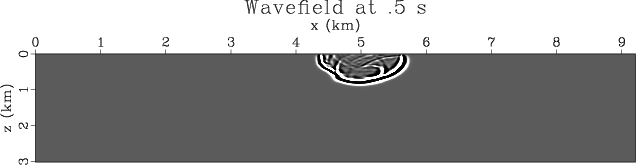
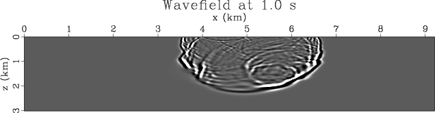
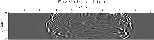
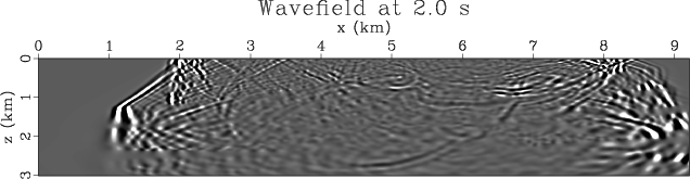
Firing the shot results the propagation of a wavefield which can be seen in the movie wfl.vpl that is generated. Typing Command 4 within the marmousi/fdmod directory displays the wavefield movie.

$$\texttt{bash-3.1\$\ scons\ wfl.vpl}$$ (4)

Four frames from this movie are presented in Figure 5 illustrating the propagation of the wavefield in the model.

time20,time40,time60,time80
Figure 5. Images of the propagating wavefield in the Marmousi model generated by a finite difference model.

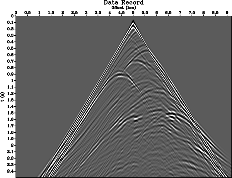
The resulting data is then presented in the file dat.vpl. This plot is reproduced here in Figure 6.

dat
Figure 6. Data gathered by the receivers in the FD model survey.

Marmousi Model