|
|
|
|
Amoco model |
| n1=384 | d1=0.0099 | o1=0 | label1=Time | unit1=s |
| n2=256 | d2=0.025 | o2=0 | label2=Offset | unit2=km |
| n3=385 | d3=0.05 | o3=0 | label3=Shot | unit3=km |
The file amoco/shots/SConstruct is presented in Table 5. This file fetches the shot data, appends the header slightly and produces several images from the record.
from rsf.proj import *
# Fetch Files from repository
Fetch("shots.hh","Amoco")
# Convert Files to RSF
Flow('shots','shots.hh', '''dd form=native |
    put  label1=time label2=offset label3=Shot unit1=km unit2=km unit3=km |
    scale rscale=.0003048''')
# Plotting Section
Result('zeroOne','shots','''window $SOURCE min2=0 max2=0 size2=1
    max3=10.6 |
    grey  pclip=96 color=I screenratio=1.5 gainpanel=a
    label2=Position label1=Time title= label3=  unit2=km unit1=s
    labelsz=6''')

Result('zeroTwo','shots','''window $SOURCE min2=0 max2=0 size2=1
    min3=10.6 |
    grey  pclip=97 color=I screenratio=1.5 gainpanel=a
    label2=Position label1=Time title= label3=  unit2=km unit1=s
    labelsz=6''')

Result('shot40','shots','''window $SOURCE  min3=14 max3=14 size3=1 |
    grey  pclip=99 color=I gainpanel=a wantframenum=y  unit1=s label1=Time
    label2=Offset unit2=km label3=Shot unit3=km title=
    screenratio=1.35 labelsz=3''')
End()
|
Typing Command 2 within the amocoshots directory runs the script.
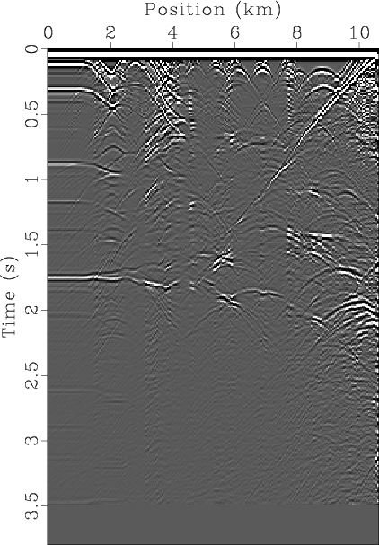
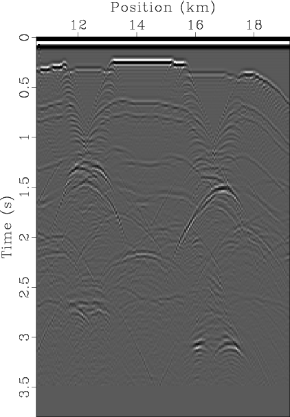
Several plots are produced. Figures 2a and 2b show the zero offset data acquired on the Amoco model. The plots are split as the large velocity contrast between the left and right side of the model muddles the image when the gainpanel filter plots the data.


|
|---|
|
zeroOne,zeroTwo
Figure 2. Amoco zero offset shot data, plot (a) goes from 0 to 10.6 km and (b) goes from 10.6 to 20 km. The plots were split as the large velocity contrast in the model makes it difficult to plot both sides on one scale. |
|
|

|
|---|
|
shot40
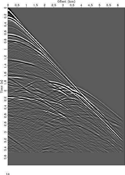
Figure 3. Amoco shot number 280; the source is 14 km from origin |
|
|
|
|
|
|
Amoco model |