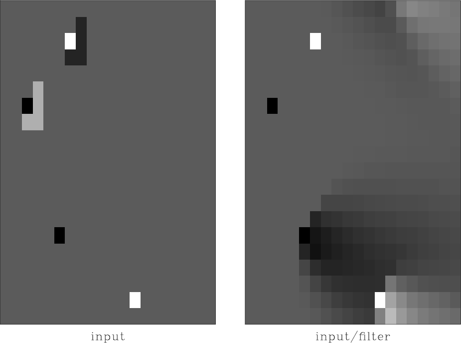
sfthreshold filters the input by soft thresholding (shrinkage).
Soft thresholding is a point-by-point operation, which can be described mathematically as
$T_{\mu}[u] = \left\{\begin{array}{rcl} u – \mu\,\mbox{sign}(u) & \quad & \mbox{if}\,|u| > \mu \\ 0 & \quad & \mbox{if}\,|u| \le \mu\end{array}\right.$
Soft thresholding was analyzed by Donoho (1995) and became particularly popular thanks to the iterative shrinkage-thresholding algorithm by Daubechies et al. (2004).
Donoho, D. L. (1995). De-noising by soft-thresholding. Information Theory, IEEE Transactions on, 41(3), 613-627.
Daubechies, I., Defrise, M., & De Mol, C. (2004). An iterative thresholding algorithm for linear inverse problems with a sparsity constraint. Communications on pure and applied mathematics, 57(11), 1413-1457.
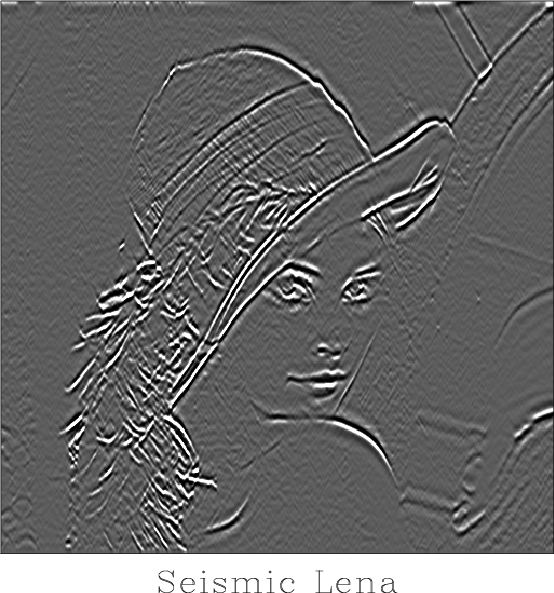
The following example from tccs/seislet/lena shows an image (Seismic Lena) and its reconstruction after soft thresholding in the seislet domain using 5% thresholding (pclip=5).
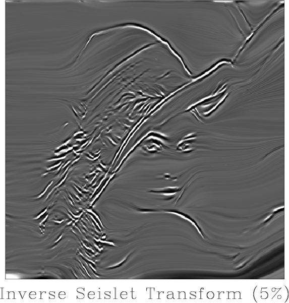
sfthreshold uses percentage parameter pclip= to set thresholding at the corresponding quantile of the data values. To do soft or hard thresholding with a fixed threshold, use sfthr.
An alternative thresholding-like operation is provided by sfsharpen.
10 previous programs of the month:

 For
For 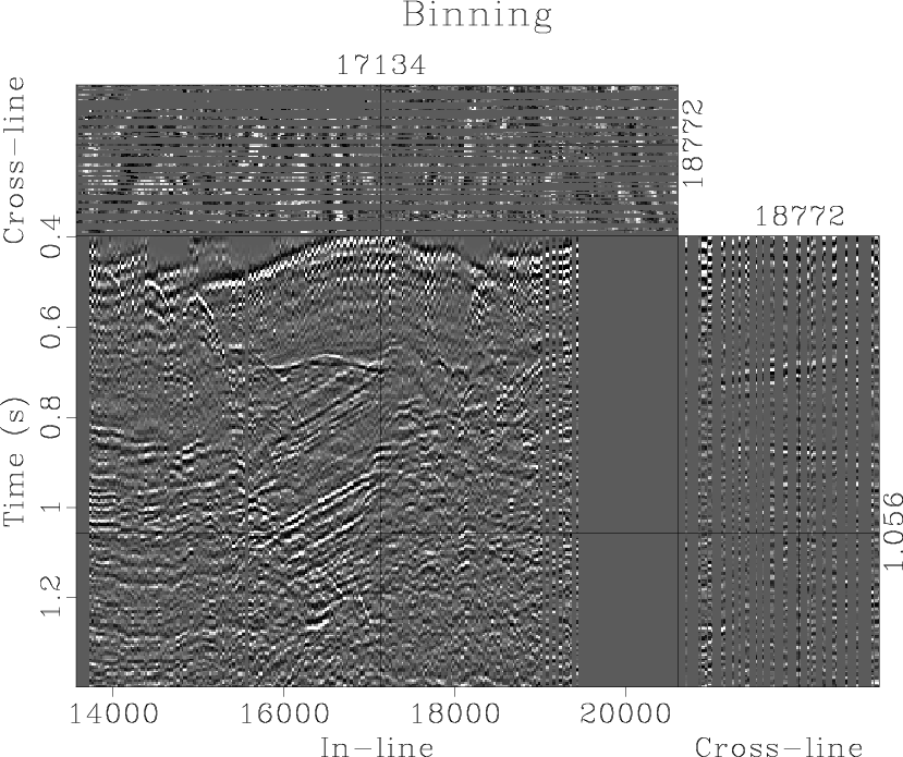 which corresponds to the following distribution of common midpoints
 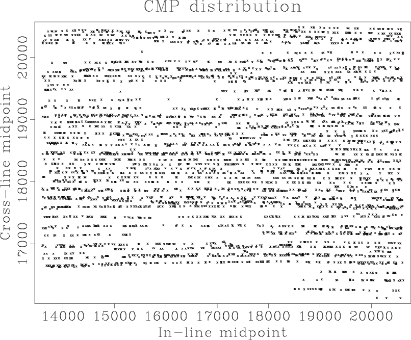 Optionally, sfbin can also output the fold map (using fold= parameter). The fold map shows the number of input traces in each output bin.
  Parameters that control output grid sampling are nx=, dx=, x0= (for the second axis), ny=, dy=, y0= (for the third axis). Alternatively, one can specify the range values xmin=, xmax=, ymin=, ymax=.