Madagascar Development Blog » 2013

Reasons not to share your code

April 22, 2013 Links No comments

In Top Ten Reasons To Not Share Your Code (and why you should anyway) published by SIAM News, Randy LeVeque, Professor of Applied Mathematics from the University of Washington, elegantly destroys common excuses computational scientists and applied mathematicians come up with when they refuse to share their software codes.

Today, most mathematicians find the idea of publishing a theorem without its proof laughable, even though many great mathematicians of the past apparently found it quite natural. Mathematics has since matured in healthy ways, and it seems inevitable that computational mathematics will follow a similar path, no matter how inconvenient it may seem. I sense growing concern among young people in particular about the way we’ve been doing things and the difficulty of understanding or building on earlier work […] We can all help our field mature by making the effort to share the code that supports our research.

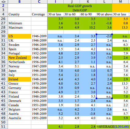
As if to illustrate LeVeque’s point, major news outlets report on a story about a reproducibility error (Excel bug) discovered in the famous politically-influential paper by economists Reinhart and Rogoff:

Reinhart, Rogoff… and Herndon: The student who caught out the profs (BBS News)
How much unemployment did Reinhart and Rogoff’s arithmetic mistake cause? (Guardian)
Is the evidence for austerity based on an Excel spreadsheet error? (Washington Post)

The validity of the Reinhart-Rogoff assertion “once debt exceeds 90 percent of GDP, economic growth drops off sharply” continues to be debated by economists, but it is clear now that their data were flawed and that the error would have been discovered much easier if the publication had followed the reproducible-research discipline.

Zooming in Vplot

April 17, 2013 Programs No comments

sfzoom is a simple Tkinter script that allows for interactive zooming when viewing Vplot files generated by sfgrey. The zoomed images are created by windowing the original RSF file and therefore have the highest possible resolution.

Joe Dellinger has a more comprehensive plan for adding interactivity to Vplot graphics.

How can I read and write RSF files in MATLAB?

April 13, 2013 FAQ No comments

The most straightforward way is to install the MATLAB interface to Madagascar. When installing Madagascar, run
```
./configure API=matlab
```
The configure script will try to find and test matlab and mex executibles on your system. If they are not in your PATH, you can specify them with
```
./configure API=matlab MATLAB=/path/to/matlab MEX=/path/to/mex
```
Install Madagascar as usual, set MATLAB path to $RSFROOT/lib, and you will able to read and write RSF files from MATLAB using rsf_read, rsf_write, and other functions from the Madagascar interface.

Alternatively, you can try reading binary data using MATLAB functions, as in the following example



% get in=, n1=, and n2= parameters from file.rsf

[stat,in] = unix(‘sfget in parform=n < file.rsf’)

in = strtrim(in)

[stat,n1] = unix(‘sfget n1 parform=n < file.rsf’)

n1 = str2num(n1)

[stat,n2] = unix(‘sfget n2 parform=n < file.rsf’)

n2 = str2num(n2)

% read binary data

fid = fopen(in,‘rb’)

data = fread(fid,n1*n2,‘float32’);

% reshape to 2-D matrix

data = reshape(data,n1,n2);

An even better alternative is to abandone MATLAB in favor of free software, such as GNU Octave, Python with NumPy, Sage, etc. A Python interface to Madagascar is installed by default.

Program of the month: sfnmo

April 8, 2013 Programs No comments

sfnmo implements normal moveout (NMO) correction, one of the most fundamental operations in seismic reflection data processing.

The following example from jsg/avo/avo shows synthetic data before and after NMO correction.

NMO transforms prestack seismic gathers by stretching each trace according to the equation
$$t = \sqrt{t_0^2 + \frac{x^2}{v^2(t_0)}}\;,$$
where $t$ is time before the correction, $t_0$ is time after the correction, $x$ is offset, and $v(t_0)$ is velocity specified in velocity= file. The NMO velocity can be picked (for example, with sfpick) from velocity scans (for example, produced with sfvscan).

If s= file is provided, sfnmo uses Malovichko’s shifted-hyperbola approximation
$$t \approx \left(1-\frac{1}{s(t_0)}\right) + \frac{1}{s(t_0)}\,\sqrt{t_0^2 + s(t_0)\,\frac{x^2}{v^2(t_0)}}$$
See

Malovichko, A. A., 1978, A new representation of the traveltime curve of reflected waves in horizontally layered media: Applied Geophysics (in Russian), 91, 47-53
Sword, C. H., 1987, A Soviet look at datum shift, in SEP-51: Stanford Exploration Project, 313-316.
de Bazelaire, E., 1988, Normal moveout revisited – Inhomogeneous media and curved interfaces: Geophysics, 53, 143-157.
Castle, R. J., 1994, Theory of normal moveout: Geophysics, 59, 983-999.

If a= file is provided, sfnmo uses Taner’s velocity-acceleration approximation
$$t = \sqrt{t_0^2 + \frac{x^2}{v^2(t_0)+a(t_0)\,x^2}}$$
See

Taner, M. T., S. Treitel, and M. Al-Chalabi, 2005, A new travel time estimation method for horizontal strata: 75th Ann. Internat. Mtg, Soc. of Expl. Geophys., 2273-2276.
Taner, M. T., S. Treitel, M. Al-Chalabi, and S. Fomel, 2007, An offset dependent NMO velocity model: EAGE 69th Conference and Exhibition, EAGE, P036.

The offset $x$ can be either regular (specified as the second axis in the input file) or irregular (specified in offset= file). By default, half-offset is used $h=x/2$. To use full offset, specify half=n.

Additionally, it is possible to specify a mask (with mask= file containing 1s and 0s) for skipping certain traces during the correction. See the following example from rsf/scons/rsf

The NMO correction is associated with the phenomenon of “NMO stretch”, a non-linear stretching of time at large offsets. The maximum allowed relative stretch is controlled by str= parameter. The part of the data that is stretched more than the allowed stretch gets muted. The width of the mute zone is controlled by mute= parameter.

NMO with constant velocity can be accomplished with sfnmostretch. For 3-D azimuthally-anisotropic moveout correction, try sfnmo3. For NMO in the tau-p domain, try sftaupmo. For an inverse NMO operation, try sfnimo.