|
|
|
|
Separation and imaging of seismic diffractions using a localized rank-reduction method with adaptively selected ranks |
Next: Automatic rank selection Up: Methods for adaptively separating Previous: Methods for adaptively separating
|
|
|
|
Separation and imaging of seismic diffractions using a localized rank-reduction method with adaptively selected ranks |
Assuming that the tensor form of the input 3D seismic data is ![]() , the corresponding form in frequency-space domain is obtained after Fourier transform and can be expressed as
, the corresponding form in frequency-space domain is obtained after Fourier transform and can be expressed as ![]() . For each frequency slice, we map the frequency domain data into several block Hankel matrices. This process is referred as Hankelization (Siahsar et al., 2017; Oropeza and Sacchi, 2011; Huang et al., 2016). Given a frequency
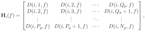
. For each frequency slice, we map the frequency domain data into several block Hankel matrices. This process is referred as Hankelization (Siahsar et al., 2017; Oropeza and Sacchi, 2011; Huang et al., 2016). Given a frequency ![]() , the Hankel matrix can be constructed as
, the Hankel matrix can be constructed as
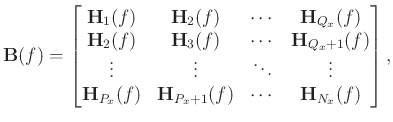
Then, the corresponding block Hankel matrix can be inserted with equation 1
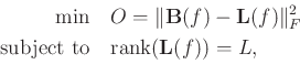
The rank-reduction can be achieved by minimizing the following objective function
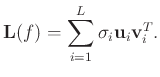
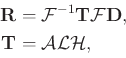
Then, the solved low-rank Hankel matrix is rearranged to a vector form according to inverse Hankelization process. The rank-reduction method can be summarized as follows:
In equation 6, filter
![]() is referred to as the frequency-domain rank-reduction operator, containing the Hankelization
is referred to as the frequency-domain rank-reduction operator, containing the Hankelization
![]() , principal component extraction
, principal component extraction
![]() and inverse Hankelization process
and inverse Hankelization process
![]() . Because of the complexity of seismic data, the plane-wave assumption is only valid locally. Thus, it is more appropriate to apply the rank-reduction method locally, i.e., in local windows:
. Because of the complexity of seismic data, the plane-wave assumption is only valid locally. Thus, it is more appropriate to apply the rank-reduction method locally, i.e., in local windows:
|
|
|
|
Separation and imaging of seismic diffractions using a localized rank-reduction method with adaptively selected ranks |