 |
 |
 |
 | A numerical tour of wave propagation |  |
![[pdf]](icons/pdf.png) |
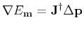
Next: Fréchet derivative
Up: Full waveform inversion (FWI)
Previous: The Newton, Gauss-Newton, and
The gradient-like method can be summarized as
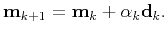 |
(80) |
The conjugate gradient (CG) algorithm decreases the misfit function along the conjugate gradient direction:
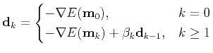 |
(81) |
There are many ways to compute  :
:
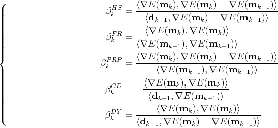 |
(82) |
To achieve best convergence rate, in practice we suggest to use a hybrid scheme combing Hestenes-Stiefel and Dai-Yuan:
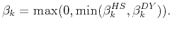 |
(83) |
Iterating with Eq. (80) needs to find an appropriate  . Here we provide two approaches to calculate
.
. Here we provide two approaches to calculate
.
 Approach 1: Currently, the objective function is
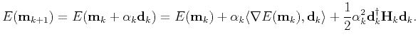 |
(84) |
Setting
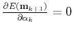 gives
gives
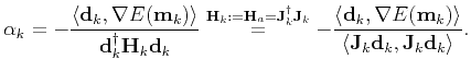 |
(85) |
Approach 2:
Recall that
 |
(86) |
Using the 1st-order approximation, we have
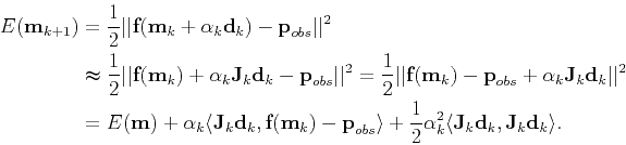 |
(87) |
Setting
gives
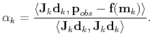 |
(88) |
In fact, Eq. (88) can also be obtained from Eq. (85) in terms of Eq. (72):
 .
.
In terms of Eq. (86), the term
 is computed conventionally using a 1st-order-accurate finite difference approximation of the partial derivative of
 :
:
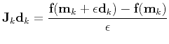 |
(89) |
with a small parameter  . In practice, we chose an
such that
. In practice, we chose an
such that
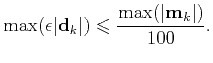 |
(90) |
|
|
|
|
| A numerical tour of wave propagation | |
|
Next: Fréchet derivative
Up: Full waveform inversion (FWI)
Previous: The Newton, Gauss-Newton, and
2021-08-31