|
|
|
|
A numerical tour of wave propagation |
Acoustics is a special case of fluid dynamics (sound waves in gases and liquids) and linear elastodynamics. Note that elastodynamics is a more accurate representation of earth dynamics, but most industrial seismic processing based on acoustic model. Recent interest in quasiacoustic anisotropic approximations to elastic P-waves.
Assume
![]() is differentiable constitutive law w.r.t. time
is differentiable constitutive law w.r.t. time ![]() .
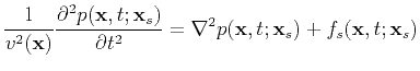
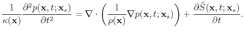
Substituting Eq. (2) into the differentiation of Eq. (1) gives
.
Substituting Eq. (2) into the differentiation of Eq. (1) gives
 |
(3) |
 |
(4) |
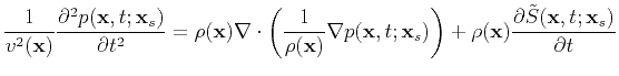
 . In 2D case, it is
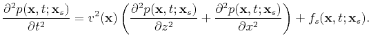 |
(6) |
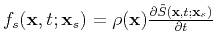
 |
(7) |
|
|---|
|
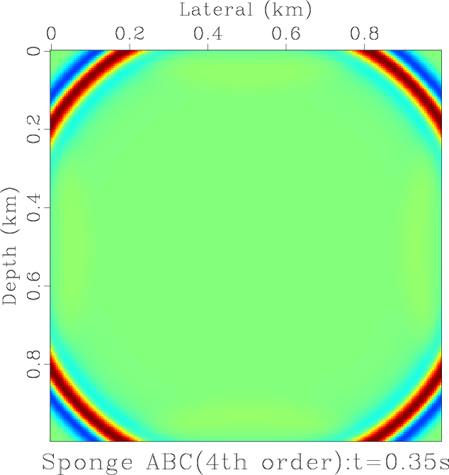
snapfd2d
Figure 1. A snap of acoustic wavefield obtained at t=0.35s with 4-th order finite difference scheme and the sponge absorbing boundary condition. |
|
|
|
|---|
|
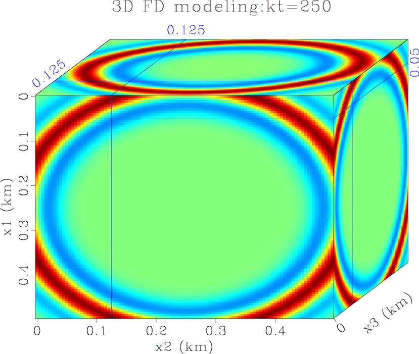
snapfd3d
Figure 2. A wavefield snap recorded at kt=250, 300 steps modeled. |
|
|
The above spatial operator is spatially homogeneous. This isotropic formula is simple and easy to understand, and becomes the basis for many complicated generalizations in which the anisotropy may come in. In 2D case, the elliptically-anisotropic wave equation reads
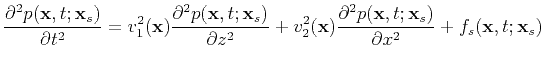 |
(8) |
|
|---|
|
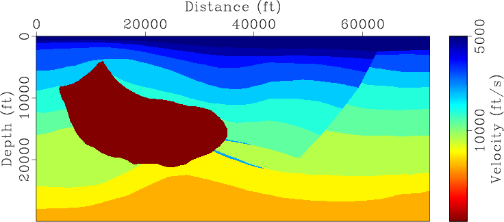
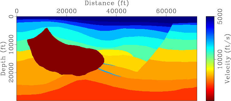
vp,vx
Figure 3. Two velocity components of Hess VTI model |
|
|
|
|---|
|
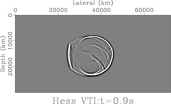
snapaniso
Figure 4. Wavefield at |
|
|
|
|
|
|
A numerical tour of wave propagation |