|
|
|
|
Simulating propagation of decoupled elastic waves using low-rank approximate mixed-domain integral operators for anisotropic media |
Then we demonstrate the approach in the 2D Hess VTI model (Figure 8).
Vertical qS-wave velocity is set to equal half the vertical qP-wave velocity everywhere.
A point-source is placed at location of (13.264, 4.023) km.
For comparison, spatial step length
![]() ft and time-step
ft and time-step
![]() ms are used in this example.
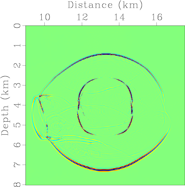
Figure 9 displays the decoupled and total displacement fields synthesized by using the low-rank pseudo-spectral algorithm
that simultaneously extrapolate the decoupled qP- and qSV-wave modes. The ranks
ms are used in this example.
Figure 9 displays the decoupled and total displacement fields synthesized by using the low-rank pseudo-spectral algorithm
that simultaneously extrapolate the decoupled qP- and qSV-wave modes. The ranks ![]() are in [8,10] for the low-rank
decomposition of the involved matrices (The ranks reduce to [1,3] if we only propagate the coupled elastic wavefields).
The wavefield snapshots show that the proposed wave propagator honors the elastic effects such as mode conversion.
It takes the CPU time of 111.6 s to decompose the mixed-domain matrices in advance, and about 9397.7 s to extrapolate the
decoupled wavefields to the maximum time of 1100.0 s.
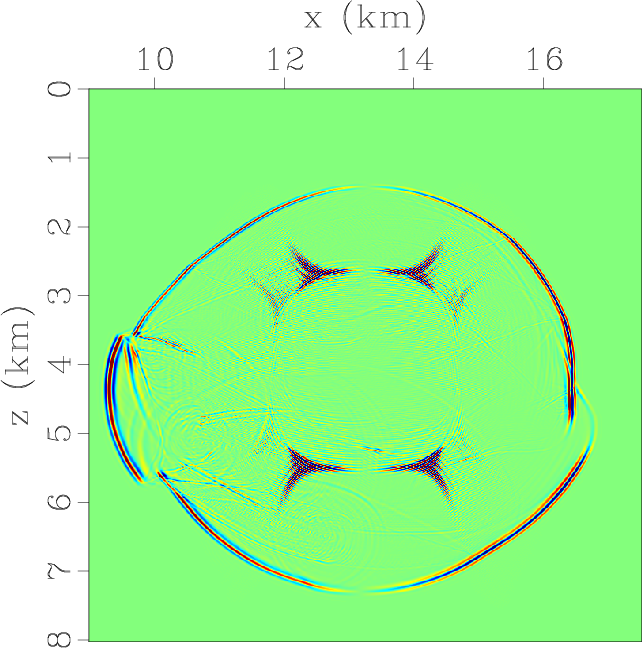
Figure 10 displays the total displacement fields synthesized by the 10th-order FD solution of the elastic
wave equation and the decoupled qP- and qSV-wave fields using the low-rank vector decomposition
for heterogeneous TI media (Cheng and Fomel, 2014).
The ranks are in
are in [8,10] for the low-rank
decomposition of the involved matrices (The ranks reduce to [1,3] if we only propagate the coupled elastic wavefields).
The wavefield snapshots show that the proposed wave propagator honors the elastic effects such as mode conversion.
It takes the CPU time of 111.6 s to decompose the mixed-domain matrices in advance, and about 9397.7 s to extrapolate the
decoupled wavefields to the maximum time of 1100.0 s.
Figure 10 displays the total displacement fields synthesized by the 10th-order FD solution of the elastic
wave equation and the decoupled qP- and qSV-wave fields using the low-rank vector decomposition
for heterogeneous TI media (Cheng and Fomel, 2014).
The ranks are in ![]() for the decomposition of the involved mode decoupling matrices
for the decomposition of the involved mode decoupling matrices ![]() .
The FD solution shows strong numerical dispersion of the qSV-waves due to inadequate
sampling because the modeling of qSV-wave using FD scheme demands finer grid cell size.
Except the CPU time of 36.7 s to decompose the mixed-domain matrices for mode decoupling,
it takes 568.0 s to extrapolate and 4690.3 s to decouple the elastic wavefields
to get qP- and qS-wave fields for all the time-steps.
To achieve the same good quality as the low-rank pseudo-spectral solution in Figure 8, we decrease the spatial
sampling to
.
The FD solution shows strong numerical dispersion of the qSV-waves due to inadequate
sampling because the modeling of qSV-wave using FD scheme demands finer grid cell size.
Except the CPU time of 36.7 s to decompose the mixed-domain matrices for mode decoupling,
it takes 568.0 s to extrapolate and 4690.3 s to decouple the elastic wavefields
to get qP- and qS-wave fields for all the time-steps.
To achieve the same good quality as the low-rank pseudo-spectral solution in Figure 8, we decrease the spatial
sampling to
![]() ft and the temporal sampling to 0.5 ms.
Except the CPU time of 133.8 s to decompose the mixed-domain matrices for mode decoupling,
it takes 3922.8 s to extrapolate and 14212.0 s to decouple the elastic wavefields to the maximum time.
This means the low-rank pseudo-spectral scheme more efficient to obtain decoupled elastic wavefields
for TI media.
ft and the temporal sampling to 0.5 ms.
Except the CPU time of 133.8 s to decompose the mixed-domain matrices for mode decoupling,
it takes 3922.8 s to extrapolate and 14212.0 s to decouple the elastic wavefields to the maximum time.
This means the low-rank pseudo-spectral scheme more efficient to obtain decoupled elastic wavefields
for TI media.


|
|---|
|
vp-hess,epsilon-hess,delta-hess
Figure 8. SEG/Hess VTI model with parameters of (a) vertical P-wave velocity, Thomsen coefficients (b) |
|
|


|
|---|
|
ElasticPxKS,ElasticPzKS,ElasticSxKS,ElasticSzKS,ElasticxKS,ElasticzKS
Figure 9. Synthesized decoupled and total displacement fields using the low-rank pseudo-spectral solution with the |
|
|


|
|---|
|
ElasticxFD,ElasticzFD,ElasticPxFD,ElasticPzFD,ElasticSxFD,ElasticSzFD
Figure 10. Elastic wavefield extrapolation using 10th-order FD scheme and low-rank vector decomposition in SEG/Hess VTI model: (a) x- and (b) z-components of the synthetic elastic displacement wavefields at 1.1 s; (c) x- and (d) z-components of vector qP-wave fields; (e) x- and (f) z-components of vector qSV-wave fields. |
|
|
|
|
|
|
Simulating propagation of decoupled elastic waves using low-rank approximate mixed-domain integral operators for anisotropic media |