A robust approach to time-to-depth conversion and interval velocity estimation from time migration in the presence of lateral velocity variations

Numerical Implementation

Below we outline the steps involved in computing one linearization update:

1. Given current $v (z,x)$, solve equation 6 for $t_0 (z,x)$ with $t_0 (0,x) = 0$;
2. Given $t_0 (z,x)$ and $x_0 (0,x) = x$, solve equation 7 for $x_0 (z,x)$;
3. Given $t_0 (z,x)$ and $x_0 (z,x)$, interpolate $v_d (z,x)$ from $v_d (t_0,x_0)$ and compute $f (z,x)$ based on equation 9;
4. Assemble linear operator B-5 and solve equation 13 for $\delta w (z,x)$.

First, we apply the fast-marching method (Sethian, 1999; Sethian and Popovici, 1999) to solve the eikonal equation 6 by initializing a plane-wave source at $z =0$. Computation for $x_0$ can be incorporated into $t_0$ by adopting the upwind finite-differences of $t_0$ for equation 7. In Figure 2, consider a currently updated grid point $C$ during forward modeling of $t_0$. If it has only one upwind neighbor $A$ that is inside the wave-front, $t_0 (C) > t_0 (A)$, then the image ray must be aligned with grid segment $AC$ and therefore $x_0 (C) = x_0 (A)$. We refer to this scenario as one-sided. If $C$ has two upwind neighbors $A$ and $B$, $t_0 (C) > \mbox{max}\{t_0 (A), t_0 (B)\}$, and they are both inside the wave-front, then the image ray must intersect the simplex $ABC$ from an angle. In this case, we compute $x_0 (C)$ from

$$\frac{(t_0 (C) - t_0 (A))(x_0 (C) - x_0 (A))}{h_z^2} + \frac{(t_0 (C) - t_0 (B))(x_0 (C) - x_0 (B))}{h_x^2} = 0\;.$$ (14)

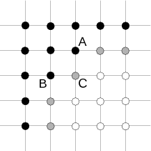
fmm
Figure 2. A modified fast-marching method for forward modeling. Black dots represent region that has been swept by the wave-front, gray dots are the expanding wave-front and grid points being updated, and white dots are region yet to be reached.

Because $\mathbf{x_0}$ at certain grid points is calculated by one-sided scenario, $\mathbf{L}_{x_0}$ there contains all zeros. Consequently, an evaluation of the cost $\mathbf{f}$ at these locations with $\mathbf{L}_{x_0} \mathbf{x_0}$ becomes inaccurate. We exclude these regions from $\mathbf{f}$ and expect inversion to fill them.

Next, we apply simple bilinear interpolation for $v_d (z,x)$ and estimate $\delta \mathbf{w}$ by solving equation 13 using shaping regularization (Fomel, 2007). We use a triangular smoother with adjustable size as the shaping operator. We find in numerical tests that shaping significantly improves convergence speed compared to that of the traditional Tikhonov regularization (Tikhonov, 1963) with gradient operators. We also observe that without regularization the model update can be undesirably oscillatory. We believe this phenomenon is related to the ill-posedness of the PDEs.

Finally, we reduce computational cost by adopting the method of conjugate gradients (Hestenes and Stiefel, 1952) and an efficient implementation of $\mathbf{J}$, as well as its adjoint, according to the equations derived in Appendix B. For this purpose, we choose the upwind finite-difference scheme (Li et al., 2011; Franklin and Harris, 2001) based on $\mathbf{t_0}$ for both $\mathbf{L}_{t_0}$ and $\mathbf{L}_{x_0}$. As shown by Li et al. (2013), applying $\mathbf{J}$ and its transpose involves only sparse triangularized matrix-vector multiplications and is therefore inexpensive. For example, at each grid point $\mathbf{L}_{t_0}^{-1}$ relies on only its upwind neighbors. The computational complexity of $\mathbf{J}$ and $\mathbf{J}^T$ is $O (N)$, where $N$ is the total number of grid points.

A robust approach to time-to-depth conversion and interval velocity estimation from time migration in the presence of lateral velocity variations