|
|
|
|
Structure-oriented singular value decomposition for random noise attenuation of seismic data |
Next: Examples Up: Theory Previous: Dip steering and local
|
|
|
|
Structure-oriented singular value decomposition for random noise attenuation of seismic data |
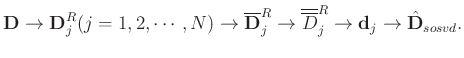
Here,
![]() denotes the
denotes the ![]() th spatial window (corresponding to
th spatial window (corresponding to ![]() th trace) with a radius of
th trace) with a radius of ![]() ,
,
![]() denotes the flattened local spatial window,
denotes the flattened local spatial window,
![]() denotes the SVD denoised local spatial window,
denotes the SVD denoised local spatial window,
![]() denotes the averaged local spatial window, and
denotes the averaged local spatial window, and
![]() denotes the output data using SOSVD.
denotes the output data using SOSVD.
As we can see from the workflow, the key step that distinguishes SOSVD with other types of SVD approaches is the flattening in the local spatial window. The flattening corresponds to applying a flattening operator to the data (here we use a prediction operator according to local slope) so that the output data have horizontal events:
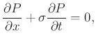
The prediction operator is a numerical solution of the local plane differential equation
The dominant slopes are estimated by solving the following least-square minimization problem using regularized least-squares optimization:
![\begin{displaymath}
\mathbf{W} = \left[
\begin{array}{ccccc}
\mathbf{I} & 0 & 0...
...hbf{P}}_{N-1\rightarrow N} & \mathbf{I}
\end{array}\right]\;,
\end{displaymath}](img60.png)
|
|
|
|
Structure-oriented singular value decomposition for random noise attenuation of seismic data |
![\begin{displaymath}\begin{split}
& \left[
\begin{array}{cccccc}
\mathbf{P}_{(1,j...
...}_{1+R,j}, \cdots, \overline{\mathbf{d}}_{1+2R,j}].
\end{split}\end{displaymath}](img51.png)