Shaping regularization in geophysical estimation problems

From triangle smoothing to triangle shaping

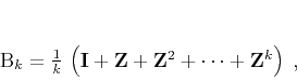
The idea of triangle smoothing can be generalized to produce different shaping operators for different applications. Let us assume that the estimated model is organized in a sequence of records, as follows: $\mathbf{m} = \left[\begin{array}{cccc} \mathbf{m}_1 & \mathbf{m}_2 & \vdots & \mathbf{m}_n \end{array}\right]^T$. Depending on the application, the records can be samples, traces, shot profiles, etc. Let us further assume that, for each pair of neighboring records, we can design a prediction operator $\mathbf{Z}_{k \rightarrow k+1}$, which predicts record $k+1$ from record $k$. A global prediction operator is then

$$\mathbf{Z} = \left[\begin{array}{cccccc} 0 & 0 & 0 & \cd... ... \mathbf{Z}_{n-1 \rightarrow n} & 0 \\ \end{array}\right]\;.$$ (14)

The operator $\mathbf{Z}$ effectively shifts each record to the next one. When local prediction is done with identity operators, this operation is completely analogous to the $Z$ operator used in the theory of digital signal processing. The $\mathbf{Z}$ operator can be squared, as follows:

$$\mathbf{Z}^2 = \left[\begin{array}{cccccc} 0 & 0 & \cdot... ...{Z}_{n-2 \rightarrow n-1} & 0 & 0 \\ \end{array}\right]\;.$$ (15)

In a shorter notation, we can denote prediction of record $j$ from record $i$ by $\mathbf{Z}_{i \rightarrow j}$ and write

$$\mathbf{Z}^2 = \left[\begin{array}{cccccc} 0 & 0 & \cdot... ...thbf{Z}_{n-2 \rightarrow n} & 0 & 0 \\ \end{array}\right]\;.$$ (16)

Subsequently, the prediction operator $\mathbf{Z}$ can be taken to higher powers. This leads immediately to an idea on how to generalize box smoothing: predict each record from the record immediately preceding it, the record two steps away, etc. and average all those predictions and the actual records. In mathematical notation, a box shaper of length $k$ is then simply

$$\mathbf{B}_k = \frac{1}{k}\,\left(\mathbf{I} + \mathbf{Z} + \mathbf{Z}^2 + \cdots + \mathbf{Z}^k\right)\;,$$ (17)

which is completely analogous to equation 7. Implementing equation 17 directly requires many computational operations. Noting that

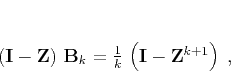$$\left(\mathbf{I} - \mathbf{Z}\right)\,\mathbf{B}_k = \frac{1}{k}\,\left(\mathbf{I} - \mathbf{Z}^{k+1}\right)\;,$$ (18)

we can rewrite equation 17 in the compact form

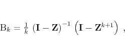$$\mathbf{B}_k = \frac{1}{k}\,\left(\mathbf{I} - \mathbf{Z}\right)^{-1}\, \left(\mathbf{I} - \mathbf{Z}^{k+1}\right)\;,$$ (19)

which can be implemented economically using recursive inversion of the lower triangular operator $\mathbf{I} - \mathbf{Z}$. Finally, combining two generalized box smoothers creates a symmetric generalized triangle shaper

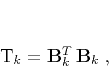$$\mathbf{T}_k = \mathbf{B}_k^T\,\mathbf{B}_k\;,$$ (20)

which is analogous to equation 8. A triangle shaper uses local predictions from both the left and the right neighbors of a record and averages them using triangle weights.

tris
Figure 3. Shaping by smoothing along local dip directions according to operator $\mathbf {T}_k$ from equation 20. a: an example image, b: local dip estimation, c: smoothing random numbers along local dips, d: impulse responses of oriented smoothing for nine different locations in the image space.

Figure 3 illustrates generalized triangle shaping by constructing a non-stationary smoothing operator that follows local structural dips. Figure 3a shows a synthetic image from Claerbout (2006). Figure 3b is a local dip estimate obtained with plane-wave destruction (Fomel, 2002). Figure 3c is the result of applying triangle smoothing oriented along local dip directions to a field of random numbers. Oriented smoothing generates a pattern reflecting the structural composition of the original image. This construction resembles the method of Claerbout and Brown (1999). Figure 3d shows the impulse responses of oriented smoothing for several distinct locations in the image space. As illustrated later in this paper, oriented smoothing can be applied for generating geophysical Earth models that are compliant with the local geological structure (Sinoquet, 1993; Clapp et al., 2004; Versteeg and Symes, 1993).

Appendix B describes general rules for combining elementary shaping operators.

Shaping regularization in geophysical estimation problems