A fast algorithm for 3D azimuthally anisotropic velocity scan

Theory

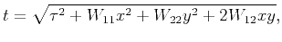
As explained by Grechka and Tsvankin (1998), a pure-mode (P or S) reflection event in an effectively azimuthally anisotropic medium can be described by

$$t=\sqrt{\tau^2+W_{11}x^2+W_{22}y^2+2W_{12}xy},$$ (1)

where $t$ is two-way CMP traveltime, $\tau$ is two-way zero-offset traveltime, $(x,y)$ is the full source-receiver offset in surface survey coordinates, and

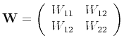$$\mathbf{W}= \left( \begin{array}{cc} W_{11} & W_{12} W_{12} & W_{22} \end{array} \right)$$ (2)

is the slowness matrix. Equation 1 follows from a truncated 2D Taylor expansion. Geometrically, it represents a curved surface that is hyperbolic in cross section and elliptic in map view.

Ideally, one can perform a semblance scan (Taner and Koehler, 1969) over the three parameters $W_{11}$ , $W_{22}$ , and $W_{12}$ simultaneously to estimate the velocity and perform NMO correction. However, this approach, if not impossible, is extremely expensive for large-size seismic data. Furthermore, since these parameters are not orthogonal, the semblance plots might appear to be extended and ambiguous, hence presenting difficulties for picking (Fowler et al., 2006).

Davidson et al. (2011) proposed a stable way of detecting azimuthal anisotropy using an orthogonal parametrization of the moveout function, which is based on an equivalent reformulation of equation 1,

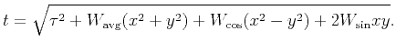$$t=\sqrt{\tau^2+W_{\text{avg}}(x^2+y^2)+W_{\cos}(x^2-y^2)+2W_{\sin}xy}.$$ (3)

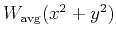
The cosine and sine dependent slownesses $W_{\cos}$ and $W_{\sin}$ are usually much smaller than the averaged slowness $W_{\text{avg}}$ . Therefore, a possible workflow for anisotropic velocity analysis and NMO correction can proceed in three steps:

1. Perform an isotropic velocity scan to estimate $W_{\text{avg}}$ and flatten seismic events.
2. Perform a residual anisotropic moveout to account for $W_{\cos}$ and $W_{\sin}$ dependent terms simultaneously.
3. Convert orthogonal parameters to more intuitive anisot-ropy parameters. For instance, the normal moveout velocity at azimuth $\alpha$ can be recovered by

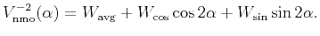   $$V_{\text{nmo}}^{-2}(\alpha)=W_{\text{avg}}+W_{\cos}\cos 2 \alpha + W_{\sin}\sin 2 \alpha.$$ (4)

   
   

In this procedure, the first two steps require a velocity-scan process. In fact, because $x$ and $y$ are symmetric in $W_{\text{avg}}(x^2+y^2)$ , the single-parameter isotropic scan involved in the first step can be handled efficiently by a 2D butterfly algorithm, as discussed in our previous work (Hu et al., 2013,2012). Our goal in this paper is to speed up the more expensive, two-parameter velocity scan in the second step.

To be specific, what we need for residual moveout is to compute a semblance as follows (assuming that the $W_{\text{avg}}$ part has been moved out from the previous step):

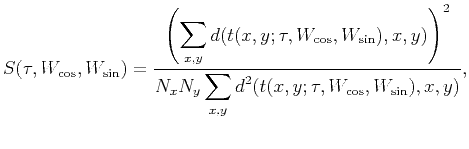$$S(\tau,W_{\cos},W_{\sin})=\frac{\left(\displaystyle\sum_{x,y}d(t(... ...right)^2}{N_xN_y\displaystyle\sum_{x,y}d^2(t(x,y;\tau,W_{\cos},W_{\sin}),x,y)},$$ (5)

where $d(t,x,y)$ is a 3D CMP dataset after isotropic moveout and

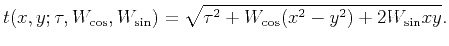$$t(x,y;\tau,W_{\cos},W_{\sin})=\sqrt{\tau^2+W_{\cos}(x^2-y^2)+2W_{\sin}xy}.$$ (6)

A fast algorithm for 3D azimuthally anisotropic velocity scan