|
 |
 |
 | Lowrank one-step wave extrapolation for reverse-time migration |  |
![[pdf]](icons/pdf.png) |
Next: Bibliography
Up: Sun et al.: Lowrank
Previous: Acknowledgments
Appendix A: Proof of the stability of one-step wave extrapolation operator
In this appendix, we prove the unconditional stability of one-step wave
extrapolation linear operator  in one-dimensional isotropic
media defined by:
in one-dimensional isotropic
media defined by:
 for for![$\displaystyle \quad f(x) \in l^2[0,1] \; ,$](img191.png) |
(47) |
where
 ,
,  is assumed to have periodic boundary
condition, and
is assumed to have periodic boundary
condition, and
 is the Fourier transform of
as
defined by equation 3. We treat
is the Fourier transform of
as
defined by equation 3. We treat  as discrete and
  as continuous for the ease of derivation. Our argument can be viewed
as a discrete version of the standard stationary phase method in the
study of pseudodifferential operators Stein (1993); Grigis and Sjöstrand (1994). To show
that the operator
as continuous for the ease of derivation. Our argument can be viewed
as a discrete version of the standard stationary phase method in the
study of pseudodifferential operators Stein (1993); Grigis and Sjöstrand (1994). To show
that the operator  is stable, a sufficient condition is that
 , where
  is a bounded constant. From
equation 47, we observe that operator
is the
composition of two operators
is a bounded constant. From
equation 47, we observe that operator
is the
composition of two operators
 , where
  is the inverse
Fourier transform and
is the inverse
Fourier transform and
 is the operator defined by:
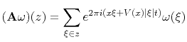 for for |
(48) |
Let us consider
 where
corresponds to a
matrix with
where
corresponds to a
matrix with  entry given by
 ,
and
,
and
 corresponds to a matrix with
  entry given by
 .
.
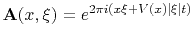
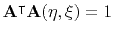
 represents a matrix with
 entry given by:
![$\displaystyle \mathbf{A}^\intercal\mathbf{A}(\eta,\xi) = \int e^{ 2\pi i[x(\xi-\eta)+V(x)(\vert\xi\vert-\vert\eta\vert)t]} dx\; .$](img213.png) |
(49) |
In order to bound the
 norm of
we
estimate the
entry of
. For
norm of
we
estimate the
entry of
. For
 ,
we have
,
we have
 . For
. For
 :
:
 |
(50) |
with
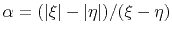 . Clearly,
 . Then
can be expressed as
. Then
can be expressed as
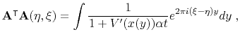
![$\displaystyle \mathbf{A}^\intercal\mathbf{A}(\eta,\xi) = \int e^{2\pi i(\xi-\eta)[x+V(x)\alpha t]}dx$](img221.png) |
(51) |
For sufficiently small  ,
,
 satisfies
![$\displaystyle \frac{1}{2} \leq \nabla_x\left[x+V(x)\alpha t\right] \leq \frac{3}{2} \; .$](img223.png) |
(52) |
Equation 51 can be expressed as:
Let us define
 . From equation 52, it is
clear that the map
. From equation 52, it is
clear that the map
 is one to one. Substituting
 into equation 53 gives
 |
(54) |
which is the inverse Fourier transform of
 . When
is small,
. When
is small,
To evaluate the norm of the integration term in the last equation, we
perform integration by part for  -times and apply periodic boundary
condition:
-times and apply periodic boundary
condition:
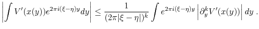 |
(56) |
Assuming sufficient smoothness on  , we have for
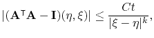 |
(57) |
for a constant C. To estimate the
norm of
 , we make use of the following lemma which can be
derived from direct calculation.
, we make use of the following lemma which can be
derived from direct calculation.
Lemma 1
Suppose
 with
with
 and
and
 , then
 is a bounded
operator.
is a bounded
operator.
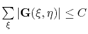
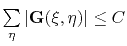
We now apply the above lemma to
 . When
 where
where  is the spatial dimension, we have
 bounded. Therefore,
for sufficiently smooth
bounded. Therefore,
for sufficiently smooth  , we have
 , for suffciently small
. Hence
, for suffciently small
. Hence
 and
and
 . Since
and
. Since
and
 as the Fourier transform
is an isometry, we have
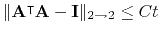
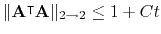
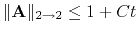
.
as the Fourier transform
is an isometry, we have
.
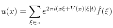
When performing wave extrapolation, fix a final time  and propagate
 steps, the operator is stable since
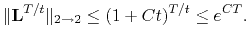 |
(58) |
|
|
|
|
| Lowrank one-step wave extrapolation for reverse-time migration | |
|
Next: Bibliography
Up: Sun et al.: Lowrank
Previous: Acknowledgments
2016-11-16
![$\displaystyle \int e^{2\pi i(\xi-\eta)[x+V(x)\alpha t]}\frac{1+V^{\prime}(x)\alpha t}{1+V^{\prime}(x)\alpha t} dx$](img225.png)
![$\displaystyle \int \frac{1}{1+V^{\prime}(x)\alpha t} e^{2\pi i(\xi-\eta)[x+V(x)\alpha t]} d\left[ x + V(x)\alpha t \right] \; .$](img226.png)
![$\displaystyle \int \left[ 1-V^{\prime}(x(y)\alpha t+\mathcal{O}(t^2)) \right]e^{2\pi i(\xi-\eta)y} dy$](img232.png)