Matching and merging high-resolution and legacy seismic images

Creating the blended image

Since the high-resolution and legacy images contain information about the same subsurface, we can attempt to create an optimal image of this area by blending the two images together to combine the strengths of each while minimizing their weaknesses. We can achieve this by imposing two conditions. First, the blended image should match the high-resolution image, particularly in the shallow part. Second, after smoothing with the non-stationary smoothing operator, the blended image should match the legacy image. 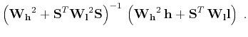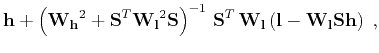We combine the two conditions together in the least-squares system

$$\left[\begin{array}{c} \mathbf{W_h} \\ \mathbf{W_lS} \end{... ...rray}{c} \mathbf{W_h\,h} \\ \mathbf{l} \end{array}\right]\;,$$ (7)

where $\mathbf{h}$ denotes the high-resolution image, $\mathbf{l}$ is the legacy image, $\mathbf{b}$ is the desired blended image, $\mathbf{W_h}$ and $\mathbf{W_l}$ are the diagonal weighting matrices for the high-resolution and legacy images, respectively, and $\mathbf{S}$ is the non-stationary smoothing specified by equation (6). The formal solution of the least-squares problem (7) is

$$\mathbf{b} = \left(\mathbf{W_h}^2 + \mathbf{S}^T\mathbf{W_l}^2\mathbf{S}\right... ...\left(\mathbf{W_h}^2\,\mathbf{h}+\mathbf{S}^T\,\mathbf{W_l}\mathbf{l}\right)\;.$$ (8)

Alternatively, equation (8) can be rearranged as

$$\mathbf{b} = \left(\mathbf{W_h}^2 + \mathbf{S}^T\mathbf{W_l}^2\mathbf{S}\right... ...T\mathbf{W_l}^2\mathbf{S}\mathbf{h}+\mathbf{S}^T\,\mathbf{W_l}\mathbf{l}\right)$$

$$= \left(\mathbf{W_h}^2 + \mathbf{S}^T\mathbf{W_l}^2\mathbf{S}\right... ...S}^T\mathbf{W_l}\left(\mathbf{l}-\mathbf{W_l}\mathbf{S}\mathbf{h}\right)\right)$$

$$= \mathbf{h} + \left(\mathbf{W_h}^2 + \mathbf{S}^T\mathbf{W_l}^2\ma... ...S}\right)^{-1}\, \mathbf{S}^T\,\mathbf{W_l}\left(\mathbf{l - W_l S h}\right)\;,$$ (9)

which makes it evident that the merged image is simply the high-resolution image with some changes.

The weights, $\mathbf{W_h}$ and $\mathbf{W_l}$, are applied to the images to bring out the desired qualities from each image. For example, since we prefer the high-resolution image in the shallow section, we weight it stronger there and gradually taper the weight to preference the legacy image with depth. In addition, we estimate the legacy weight, $\mathbf{W_l}$, to balance the legacy images's amplitudes with respect to the high-resolution image. The specific values we used for the weights are shown in Figure 6.

hweight,lweight-reverse
Figure 6. The weights for the high-resolution (a) and legacy (b) images for the least-squares merge. The high-resolution weight is strongly weighted in the shallow part and blends to favor the legacy image with depth. The legacy weight is selected to boost the legacy image's amplitudes to match that of the high-resolution image.

nspectra22-reverse
Figure 7. The spectra of the entire image display of the legacy (red dashed), high-resolution (blue dotted), and merged (magenta solid) images for the first data set.

We implement the inversion in equation (9) iteratively using the method of conjugate gradients (Hestenes and Stiefel, 1952). The resultant blended image, shown in Figure 1c, retains the higher frequencies from the high-resolution image while incorporating the lower frequencies from the legacy image (Figure 7). The broader frequency bandwidth corresponds to an increase in resolution and leads to a more detailed and interpretable image. As a result, the blended image resembles the high-resolution image but has a marked decrease in noise and extended coverage with depth.

Although the method presented in this paper is applied to post-stack images, the general method is likely flexible enough to be extended to pre-stack data. Applications of matching legacy and high-resolution seismic data are also seen in time-lapse image registration, where the accurate interpretation of 4D time-lapse data heavily depends on dataset alignment and uniform processing (Ross and Altan, 1997). The method from this paper could also be used in 4D time-lapse processing; particularly the steps involving frequency balancing and accounting for time shifts.

Matching and merging high-resolution and legacy seismic images